The objective of this chapter is to identify the optimal ARMA(p,q) model to describe the dynamics of ASML log-returns. To determine the most suitable stochastic process, we adopt a systematic approach structured in the following stages:
Exploratory Analysis: Analysis of autocorrelation functions (ACF/PACF) to assess temporal dependency and detect potential seasonality or distinct patterns.
Model Selection (Grid Search): Estimation of various order combinations, residual analysis (plots and Ljung-Box test), and selection of the “winning” models based on the minimization of AIC (Akaike Information Criterion) and BIC (Bayesian Information Criterion).
Out-of-Sample Validation: Comparison of the predictive performance of the selected models against a benchmark (historical mean) using a test set withheld from the estimation process.
2.1 ACF and PACF Analysis
Analyzing correlograms is the preliminary step to identify potential orders for the AR (AutoRegressive) and MA (Moving Average) components.
Code
acf_res <-acf(log_returns$LogReturns, plot =FALSE, lag.max =20)pacf_res <-pacf(log_returns$LogReturns, plot =FALSE, lag.max =20)ci <-qnorm((1+0.95)/2)/sqrt(length(log_returns$LogReturns))df_acf <-data.frame(lag =as.numeric(acf_res$lag)[-1],acf =as.numeric(acf_res$acf)[-1])df_pacf <-data.frame(lag =as.numeric(pacf_res$lag),pacf =as.numeric(pacf_res$acf))fig_acf <-plot_ly(df_acf, x =~lag, y =~acf, type ='bar', name ='ACF',marker =list(color ='#1f77b4')) %>%add_segments(x =min(df_acf$lag), xend =max(df_acf$lag), y = ci, yend = ci, line =list(color ='red', dash ='dash', width =1), showlegend =FALSE) %>%add_segments(x =min(df_acf$lag), xend =max(df_acf$lag), y =-ci, yend =-ci, line =list(color ='red', dash ='dash', width =1), showlegend =FALSE) %>%layout(yaxis =list(title ="ACF"))fig_pacf <-plot_ly(df_pacf, x =~lag, y =~pacf, type ='bar', name ='PACF',marker =list(color ='#ff7f0e')) %>%add_segments(x =min(df_pacf$lag), xend =max(df_pacf$lag), y = ci, yend = ci, line =list(color ='red', dash ='dash', width =1), showlegend =FALSE) %>%add_segments(x =min(df_pacf$lag), xend =max(df_pacf$lag), y =-ci, yend =-ci, line =list(color ='red', dash ='dash', width =1), showlegend =FALSE) %>%layout(yaxis =list(title ="PACF"))subplot(fig_acf, fig_pacf, nrows =1, margin =0.05, titleY =TRUE) %>%layout(title ="Autocorrelation & Partial Autocorrelation", margin =list(t =50))
Log-Returns ACF and PACF
Observations: The autocorrelation at lag-1 is statistically significant, yet its magnitude is limited (approximately -0.04). Neither the ACF nor the PACF exhibits a clear decay or a sharp cutoff. This ambiguity makes it difficult to visually identify a pure AR or MA process, suggesting instead a mixed ARMA structure.
A classical iterative approach (“Box-Jenkins”) would proceed by analyzing the residuals:
If the residuals’ ACF shows a sharp cutoff \(\rightarrow\) add an MA term.
If the residuals’ PACF shows a sharp cutoff \(\rightarrow\) add an AR term.
If both plots decay slowly or are unclear \(\rightarrow\) increase both orders.
However, given the ambiguity of the observed patterns and considering that high-order lags (\(>3\)) are uncommon in financial contexts, we opted for a more transparent and systematic approach. We will perform a comprehensive search, testing all possible combinations within a limited range.
2.2 Models
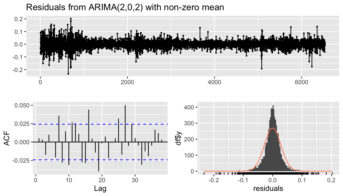
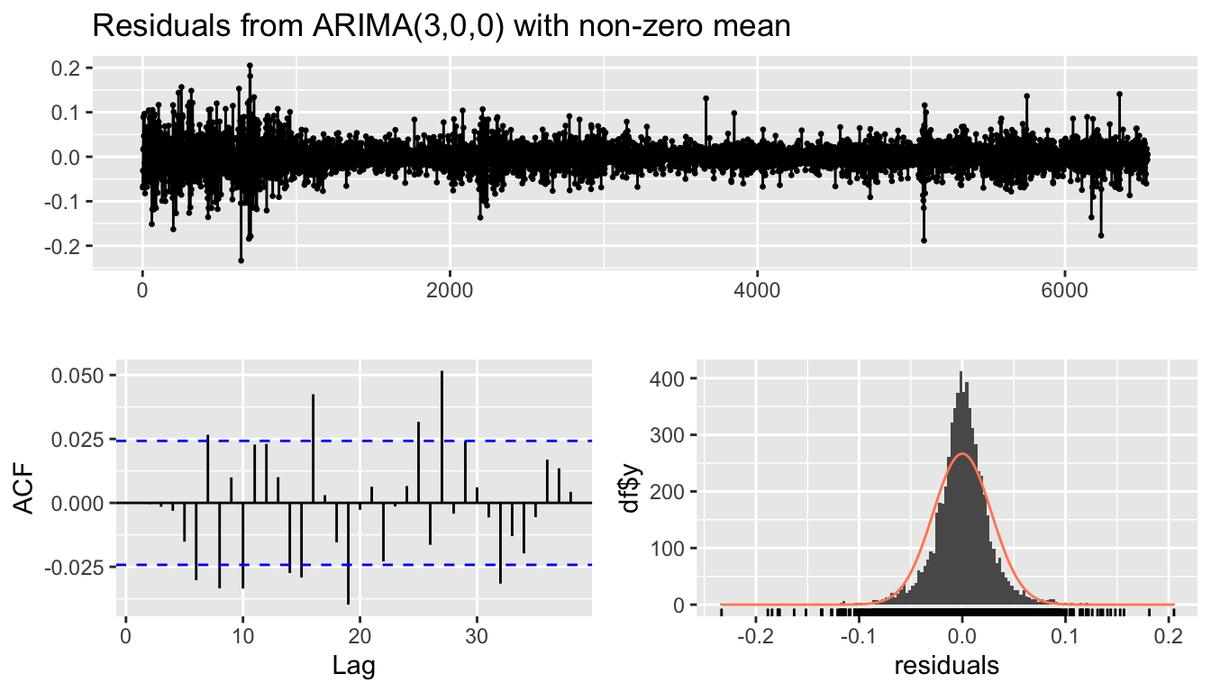
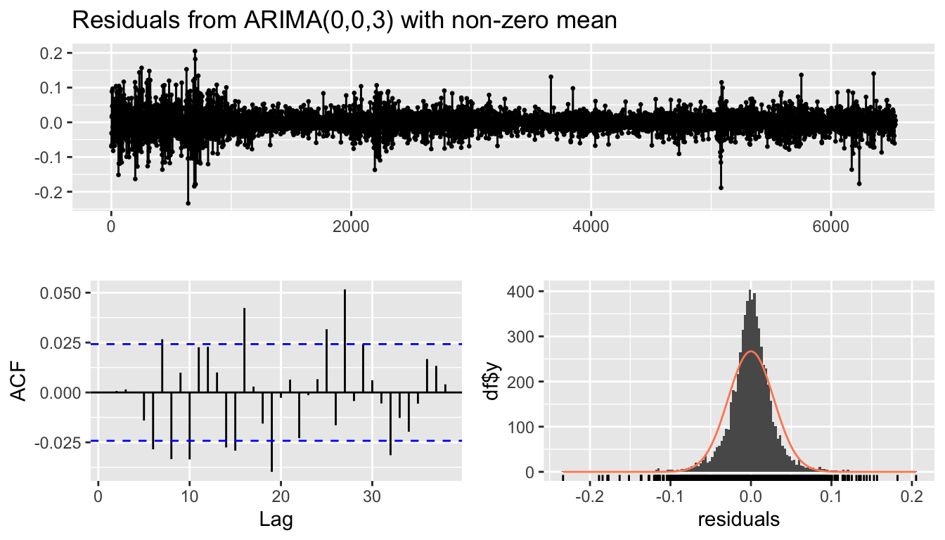
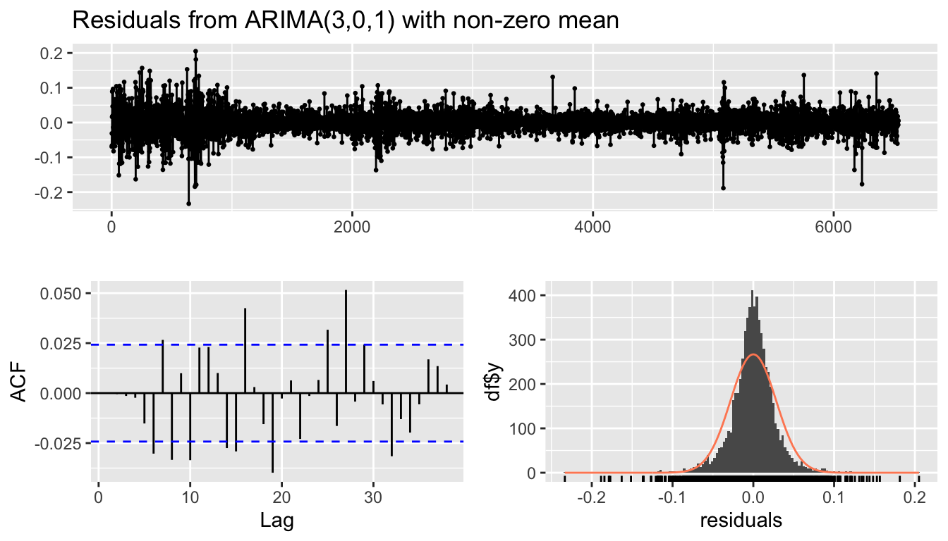
To assess the goodness of fit for each configuration, we analyze two fundamental diagnostic outputs:
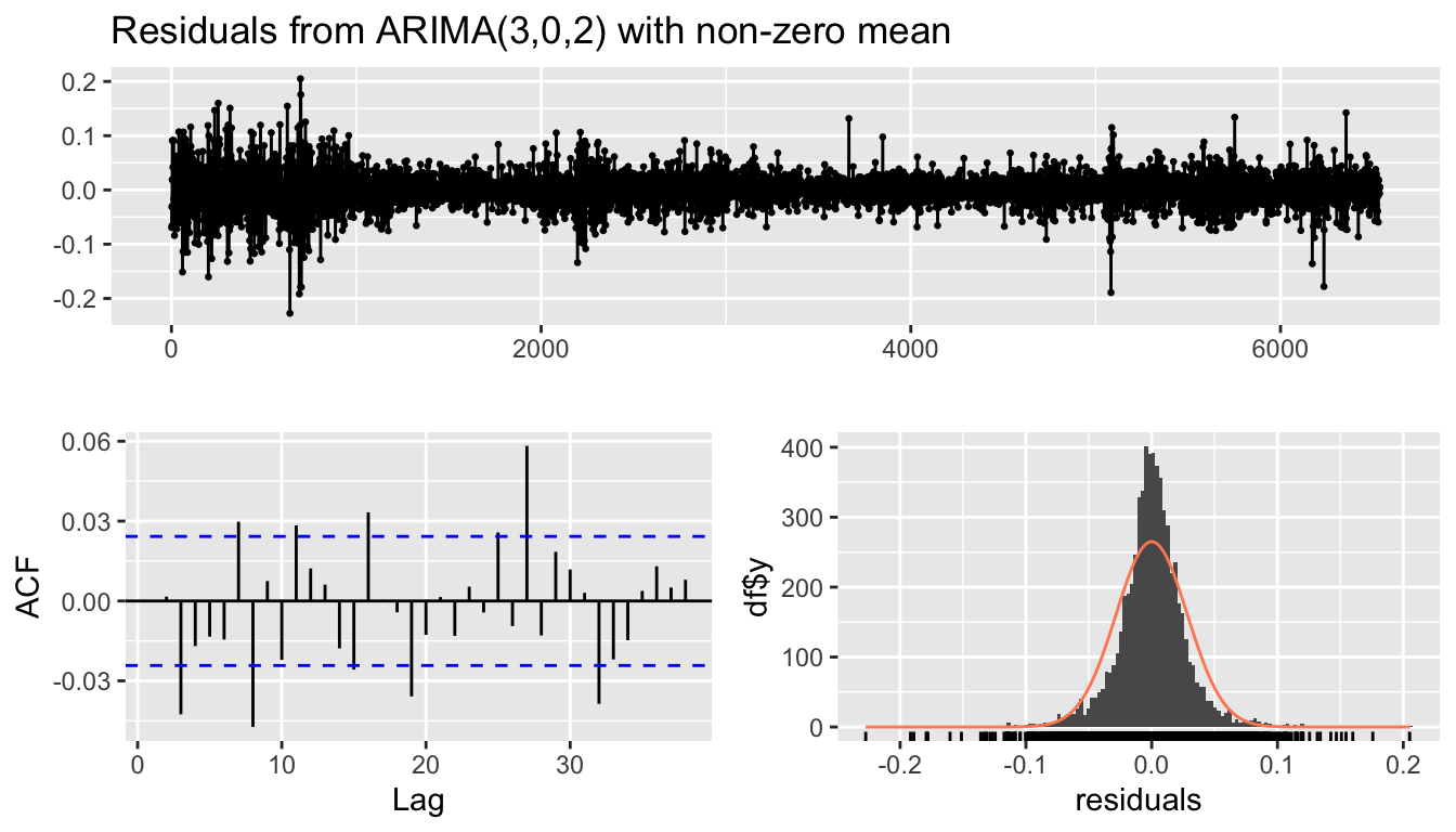
Residual Analysis (checkresiduals): This function allows us to verify the absence of autocorrelation in the residuals. In addition to a visual inspection of the plots, the Ljung-Box Test is performed.
\(H_0\) (Null Hypothesis): The residuals are independently distributed (White Noise).
Interpretation: A p-value \(>0.05\) indicates that there is insufficient evidence to reject the null hypothesis. Therefore, the model has adequately captured the temporal structure of the data.
Parameter Significance (coeftest): This reports the estimated coefficients (ar and ma) along with their Standard Errors. Using the z-test, we verify whether the coefficients are statistically different from zero (p-value \(<0.05\)).
    Ljung-Box test

data:  Residuals from ARIMA(1,0,3) with non-zero mean
Q* = 27.07, df = 6, p-value = 0.0001405

Model df: 4.   Total lags used: 10
Code
coeftest(arma_13)
Warning in sqrt(diag(se)): NaNs produced
z test of coefficients:

             Estimate  Std. Error z value Pr(>|z|)
ar1        0.33895106         NaN     NaN      NaN
ma1       -0.37787376         NaN     NaN      NaN
ma2       -0.00033557         NaN     NaN      NaN
ma3       -0.03535024         NaN     NaN      NaN
intercept  0.00051530  0.00031168  1.6533  0.09828 .
---
Signif. codes:  0 '***' 0.001 '**' 0.01 '*' 0.05 '.' 0.1 ' ' 1
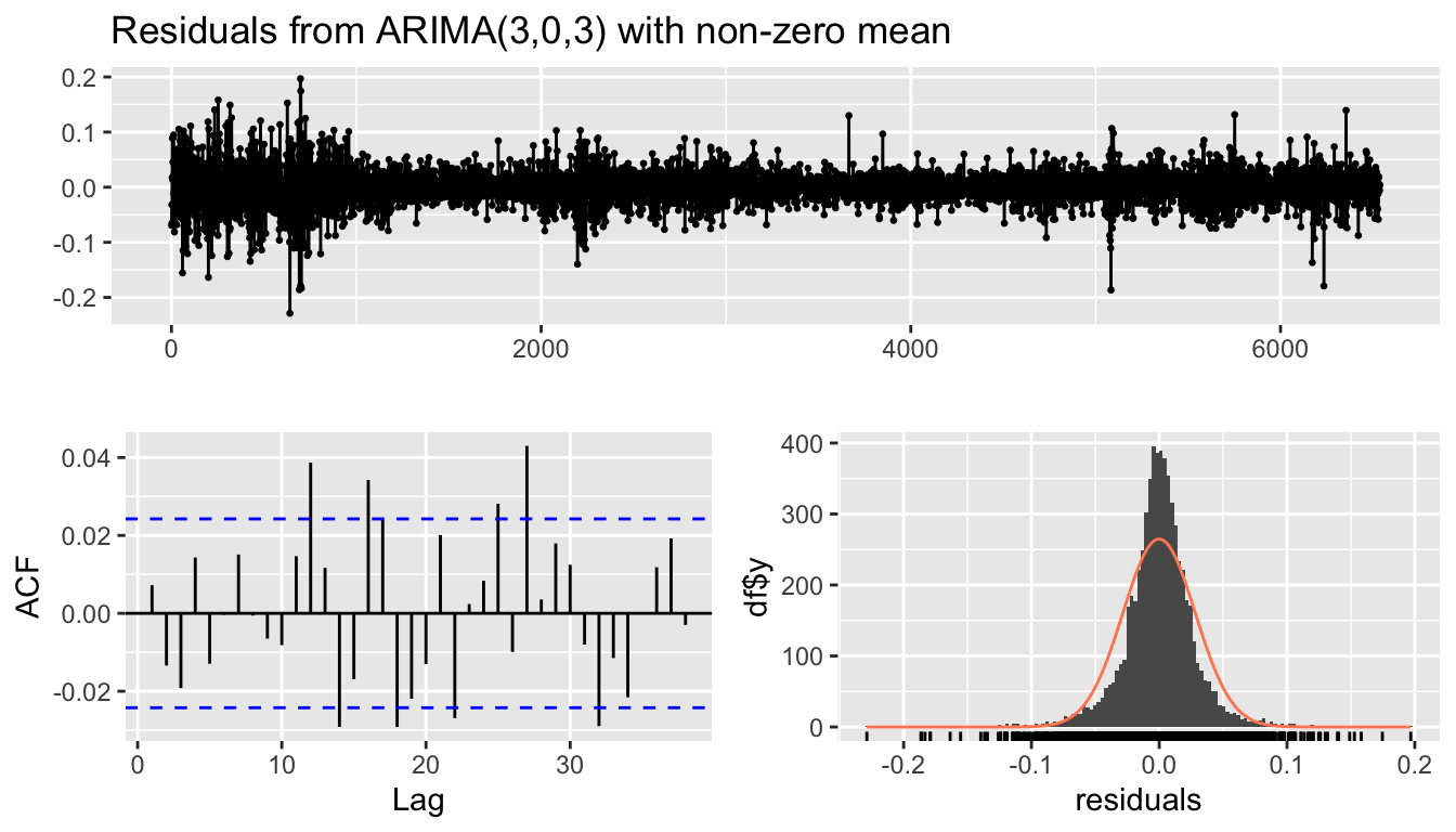
    Ljung-Box test

data:  Residuals from ARIMA(3,0,3) with non-zero mean
Q* = 8.5727, df = 4, p-value = 0.07271

Model df: 6.   Total lags used: 10
Code
coeftest(arma_33)
Warning in sqrt(diag(se)): NaNs produced
z test of coefficients:

             Estimate  Std. Error  z value Pr(>|z|)
ar1       -0.93303265         NaN      NaN      NaN
ar2        0.68686580  0.06141265  11.1844  < 2e-16 ***
ar3        0.81111732  0.07456554  10.8779  < 2e-16 ***
ma1        0.89063594         NaN      NaN      NaN
ma2       -0.72881204  0.05908310 -12.3354  < 2e-16 ***
ma3       -0.80508569  0.07150341 -11.2594  < 2e-16 ***
intercept  0.00060076  0.00028783   2.0872  0.03687 *
---
Signif. codes:  0 '***' 0.001 '**' 0.01 '*' 0.05 '.' 0.1 ' ' 1
As observed from the outputs, the simpler models (such as AR(1) and MA(1)) yield very low p-values for the Ljung-Box test (\(<0.05\)). This indicates that significant autocorrelation remains within the residuals, implying that these models have failed to capture all the relevant information.
Conversely, as we increase complexity towards an ARMA(3,3), the p-value rises above the critical 5% threshold. Consequently, we fail to reject the null hypothesis: the residuals of this model behave as White Noise. This suggests that the ARMA(3,3) is mathematically effective in capturing the patterns of the time series, although its high complexity warrants caution regarding the risk of overfitting.
Additionally, the ARMA(1,3) model exhibits instability in parameter estimation (incalculable Std. Error), pointing to potential over-parameterization.
2.3 AIC vs BIC
We visualize the trends of the information criteria for all estimated models.
Code
models_list <-list("AR(1)"= arma_10, "MA(1)"= arma_01, "ARMA(1,1)"= arma_11,"AR(2)"= arma_20, "MA(2)"= arma_02, "ARMA(1,2)"= arma_12,"ARMA(2,1)"= arma_21, "ARMA(2,2)"= arma_22,"AR(3)"= arma_30, "MA(3)"= arma_03, "ARMA(1,3)"= arma_13,"ARMA(2,3)"= arma_23, "ARMA(3,1)"= arma_31, "ARMA(3,2)"= arma_32,"ARMA(3,3)"= arma_33)metrics_df <-data.frame(Model =names(models_list),AIC =sapply(models_list, AIC),BIC =sapply(models_list, BIC))metrics_df$Model <-factor(metrics_df$Model, levels = metrics_df$Model)min_aic_val <-min(metrics_df$AIC)min_bic_val <-min(metrics_df$BIC)plot_aic <-plot_ly(metrics_df, x =~Model, y =~AIC, name ='AIC',type ='scatter', mode ='lines+markers',line =list(color ='#1f77b4', width =2),marker =list(size =8, color ='#1f77b4')) %>%layout(title ="AIC Trend", yaxis =list(title ="AIC"))best_aic <- metrics_df[metrics_df$AIC == min_aic_val, ]plot_aic <- plot_aic %>%add_trace(data = best_aic, x =~Model, y =~AIC, type ='scatter', mode ='markers', name ='Best AIC',marker =list(color ='red', size =12, symbol ='star'),showlegend =FALSE )plot_bic <-plot_ly(metrics_df, x =~Model, y =~BIC, name ='BIC',type ='scatter', mode ='lines+markers',line =list(color ='#ff7f0e', width =2),marker =list(size =8, color ='#ff7f0e')) %>%layout(title ="BIC Trend", yaxis =list(title ="BIC"))best_bic <- metrics_df[metrics_df$BIC == min_bic_val, ]plot_bic <- plot_bic %>%add_trace(data = best_bic, x =~Model, y =~BIC, type ='scatter', mode ='markers', name ='Best BIC',marker =list(color ='red', size =12, symbol ='star'),showlegend =FALSE )final_plot <-subplot(plot_aic, plot_bic, nrows =2, shareX =TRUE, titleY =TRUE) %>%layout(title ="Model Selection Criteria: AIC & BIC Trends",hovermode ="x unified",margin =list(t =50) )final_plot
Comparison between AIC and BIC
The graphical analysis of the information criteria highlights a typical divergence found in financial time series modeling.
As evidenced by the plot, the AIC criterion, which prioritizes goodness of fit, identifies the ARMA(3,3) as the optimal model (minimum value). Conversely, the BIC criterion, which penalizes model complexity more severely to prevent overfitting, suggests a much more parsimonious model: the ARMA(1,1).
Faced with these conflicting indications (a complex model vs a simple model), it is not possible to determine a priori which one is superior. To resolve this ambiguity and assess which model generalizes better on unobserved data, we will proceed with an Out-of-Sample validation, computing forecasts and comparing error metrics against actual data.
2.4 Forecast
Since the information criteria (AIC and BIC) suggest different models, we proceed with an Out-of-Sample validation to test the actual predictive capacity on data not used for estimation.
We split the time series into two subsets:
Training Set (\(80\%\)): Used to estimate the model parameters.
Test Set (\(20\%\)): Used to compare forecasts against actual data (h-step-ahead forecast).
The following plot displays the time series trend and the forecasts generated by the three models over the test period.
Note
Given the stationary nature and high volatility of log-returns, it is expected that medium-to-long-term forecasts will tend to converge rapidly towards the unconditional mean of the process. For this reason we apply method as one-step-ahead and k-step-ahead.
fit_bic_rolling <-Arima(log_returns$LogReturns, model = mod_winner_bic)one_step_bic <-fitted(fit_bic_rolling)[(n_train +1):n_total]fit_aic_rolling <-Arima(log_returns$LogReturns, model = mod_winner_aic)one_step_aic <-fitted(fit_aic_rolling)[(n_train +1):n_total]dates_test <- log_returns$Date[(n_train +1):n_total]fig_roll <-plot_ly(x = dates_test, y = test_data, type ='scatter', mode ='lines', name ='Actual Test Data', line =list(color ='black', width =1, dash ='dot'))fig_roll <-add_trace( fig_roll, x = dates_test, y =as.numeric(one_step_bic), name ='Rolling ARMA(1,1)', line =list(color ='blue', width =1))fig_roll <-add_trace( fig_roll, x = dates_test, y =as.numeric(one_step_aic), name ='Rolling ARMA(3,3)', line =list(color ='red', width =1))fig_roll <-layout( fig_roll,title ="One-Step-Ahead Rolling Forecast (Test Set: 20%)",xaxis =list(title ="Date"),yaxis =list(title ="Log Return"),legend =list(orientation ="h", x =0.1, y =-0.2))fig_roll
Comparison One-Step-Ahead Rolling Forecast
Code
calc_k_step_rolling <-function(model_obj, series, n_train, k=5) { n_total <-length(series) test_indices <- (n_train +1):n_total forecasts <-numeric(length(test_indices))for (i inseq_along(test_indices)) { target_idx <- test_indices[i] origin_idx <- target_idx - kif (origin_idx >0) { subset_data <- series[1:origin_idx] fit_temp <-Arima(subset_data, model = model_obj) fc_temp <-forecast(fit_temp, h = k) forecasts[i] <-as.numeric(fc_temp$mean[k]) } else { forecasts[i] <-NA } }return(forecasts)}k_horizon <-5vec_5step_bic <-calc_k_step_rolling(mod_winner_bic, log_returns$LogReturns, n_train, k = k_horizon)vec_5step_aic <-calc_k_step_rolling(mod_winner_aic, log_returns$LogReturns, n_train, k = k_horizon)dates_test <- log_returns$Date[(n_train +1):n_total]fig_roll_5 <-plot_ly(x = dates_test, y = test_data, type ='scatter', mode ='lines', name ='Actual Test Data', line =list(color ='black', width =1, dash ='dot'))fig_roll_5 <-add_trace( fig_roll_5, x = dates_test, y = vec_5step_bic, name ="Rolling ARMA(1,1)", line =list(color ='blue', width =1.5))fig_roll_5 <-add_trace( fig_roll_5, x = dates_test, y = vec_5step_aic, name ="Rolling ARMA(3,3)", line =list(color ='red', width =1.5))fig_roll_5 <-layout( fig_roll_5,title ="Five-Step-Ahead Rolling Forecast (Test Set: 20%)",xaxis =list(title ="Date"),yaxis =list(title ="Log Return"),legend =list(orientation ="h", x =0.1, y =-0.2))fig_roll_5
Comparison Five-Step-Ahead Rolling Forecast
We evaluate the predictive performance using:
MAE (Mean absolute Error)
RMSE (Root Mean Squared Error)
Theil’s U2 index: The ratio between the model’s RMSE and the Naive model’s RMSE.
\(U<1\): The model outperforms the benchmark.
\(U \approx 1\): The model performs equivalently to the benchmark.
\(U>1\): The model performs worse than the benchmark.
As highlighted in the table, the Theil’s U2 index for both ARMA models is extremely close to 1. This indicates that the statistical models, despite their complexity, fail to significantly outperform the simple forecast based on the historical mean (Naive Benchmark).
Important
This result is consistent with the Efficient Market Hypothesis (EMH), according to which past returns contain little to no useful information for predicting future short-term returns, making the series resemble a Random Walk.
2.5 Conclusion
The analysis conducted in this chapter has highlighted the limitations of stationary linear models in forecasting the direction of ASML returns.
Although information criteria (AIC) identified the ARMA(3,3) as a mathematical structure capable of “whitening” the in-sample residuals, the Out-of-Sample validation delivered an unequivocal verdict: a Theil’s U index close to 1 confirms that no ARMA model systematically outperforms the Naive benchmark. This empirical result corroborates the hypothesis that, regarding the conditional mean, returns follow a process closely resembling a Random Walk, rendering trading strategies based solely on past autocorrelation futile.
However, the unpredictability of the mean does not imply a total absence of structure within the series. Visual inspection of the log-returns plot reveals evident volatility clustering: periods of high volatility tend to be followed by high volatility, and periods of calm by calm (a phenomenon known as conditional heteroskedasticity).
By assuming constant variance over time (homoskedasticity), ARMA models fail to capture this fundamental characteristic of financial markets. Therefore, in the next chapter, we will shift our focus from predicting the sign of returns to modeling their magnitude (risk) by introducing the GARCH (Generalized AutoRegressive Conditional Heteroskedasticity) family of models.