2 Univariate Analysis
Private
As we can see in the bar plot above, the binary variable “Private” is unbalanced, with about 73% of colleges being private and about 27% public.
Applications
Distribution Fitting
## *******************************************************************
## Family:  c("GIG", "Generalised Inverse Gaussian")
##
## Call:  gamlssML(formula = y, family = DIST[i])
##
## Fitting method: "nlminb"
##
##
## Coefficient(s):
##             Estimate  Std. Error   t value Pr(>|t|)
## eta.mu     8.0069136   0.0475550 168.37166  < 2e-16 ***
## eta.sigma  0.3207699   0.0349293   9.18341  < 2e-16 ***
## eta.nu    -0.3138488   0.1163661  -2.69708 0.006995 **
## ---
## Signif. codes:  0 '***' 0.001 '**' 0.01 '*' 0.05 '.' 0.1 ' ' 1
##
##  Degrees of Freedom for the fit: 3 Residual Deg. of Freedom   774
## Global Deviance:     13834.8
##             AIC:     13840.8
##             SBC:     13854.7
##
## Asymptotic one-sample Kolmogorov-Smirnov test
##
## data: unique(variable)
## D = 0.031509, p-value = 0.4803
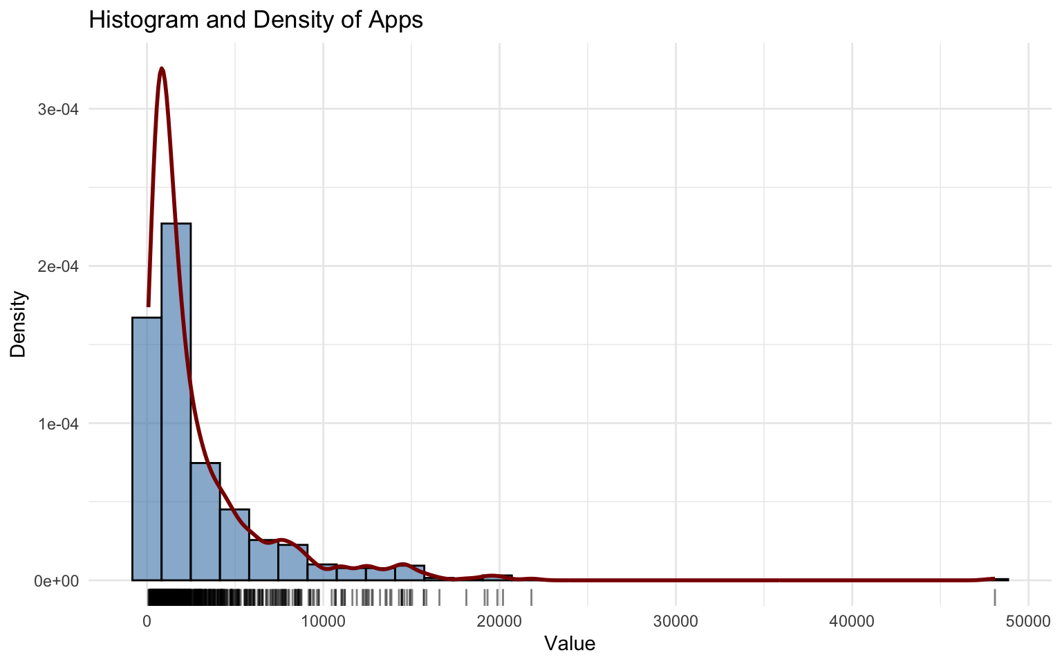
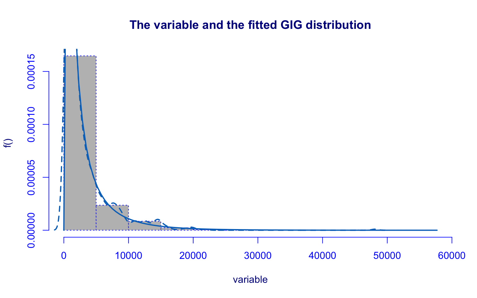
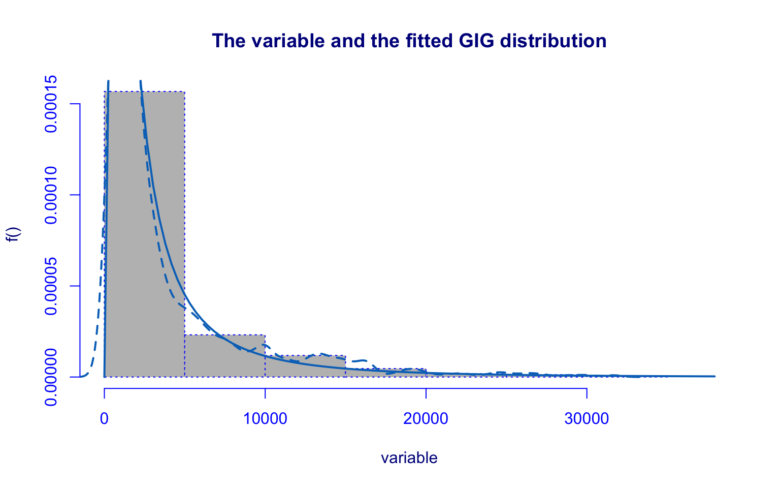
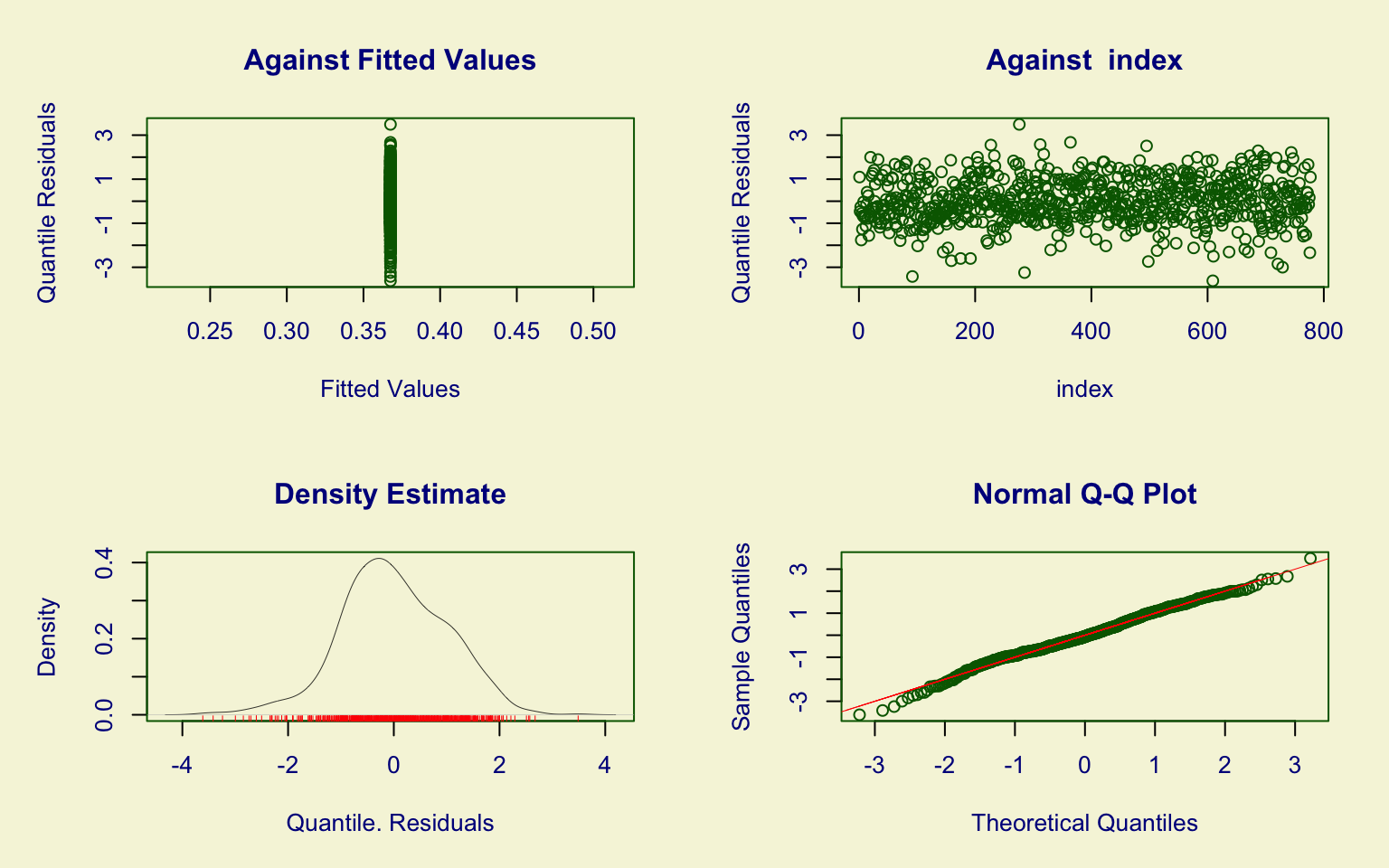
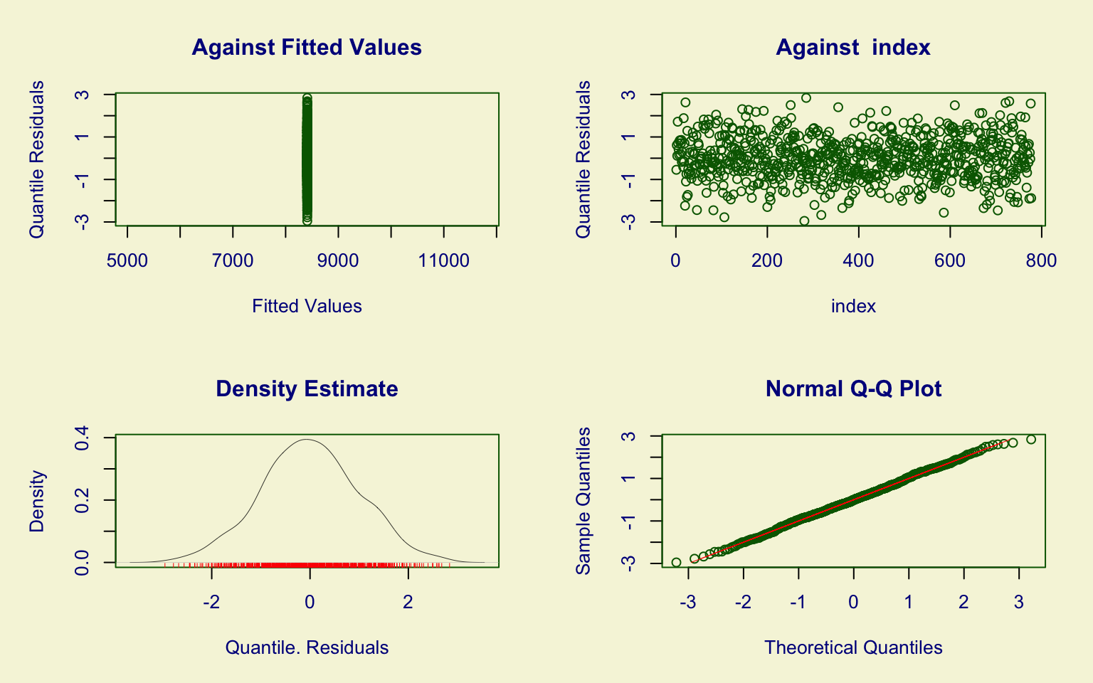
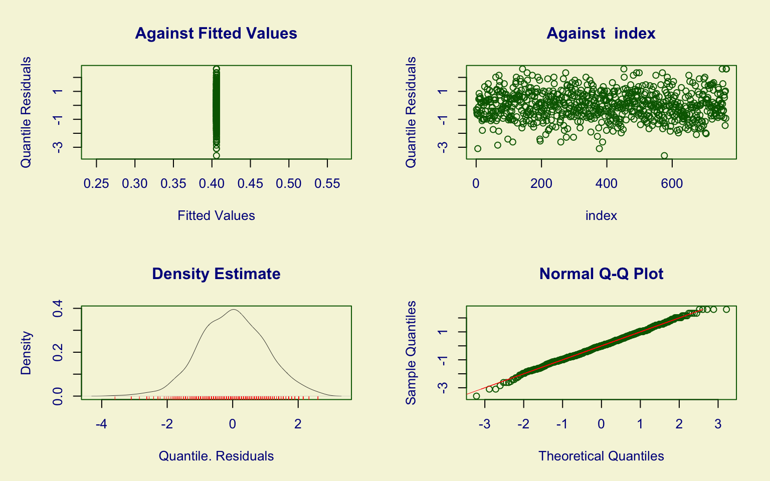
## alternative hypothesis: two-sidedThe Apps variable shows a highly right-skewed distribution with several high-value outliers. The boxplot reveals that most institutions received a relatively low number of applications, while some colleges stand out with exceptionally high values, in some cases exceeding 20,000, with one extreme case near 50,000.
The histogram with KDE estimation highlights the strong concentration in the lower range and the presence of a long right tail. The distribution fitted using the Generalized Inverse Gaussian (GIG) model provides a good approximation, capturing both the skewness and the general shape of the distribution.
The estimates of \(\hat\mu\) and \(\hat\sigma\) are more significant, with values of about 8 and 0.32. The \(\hat\nu\) is slightly less significant than others parameters, with a value of about -0.31.
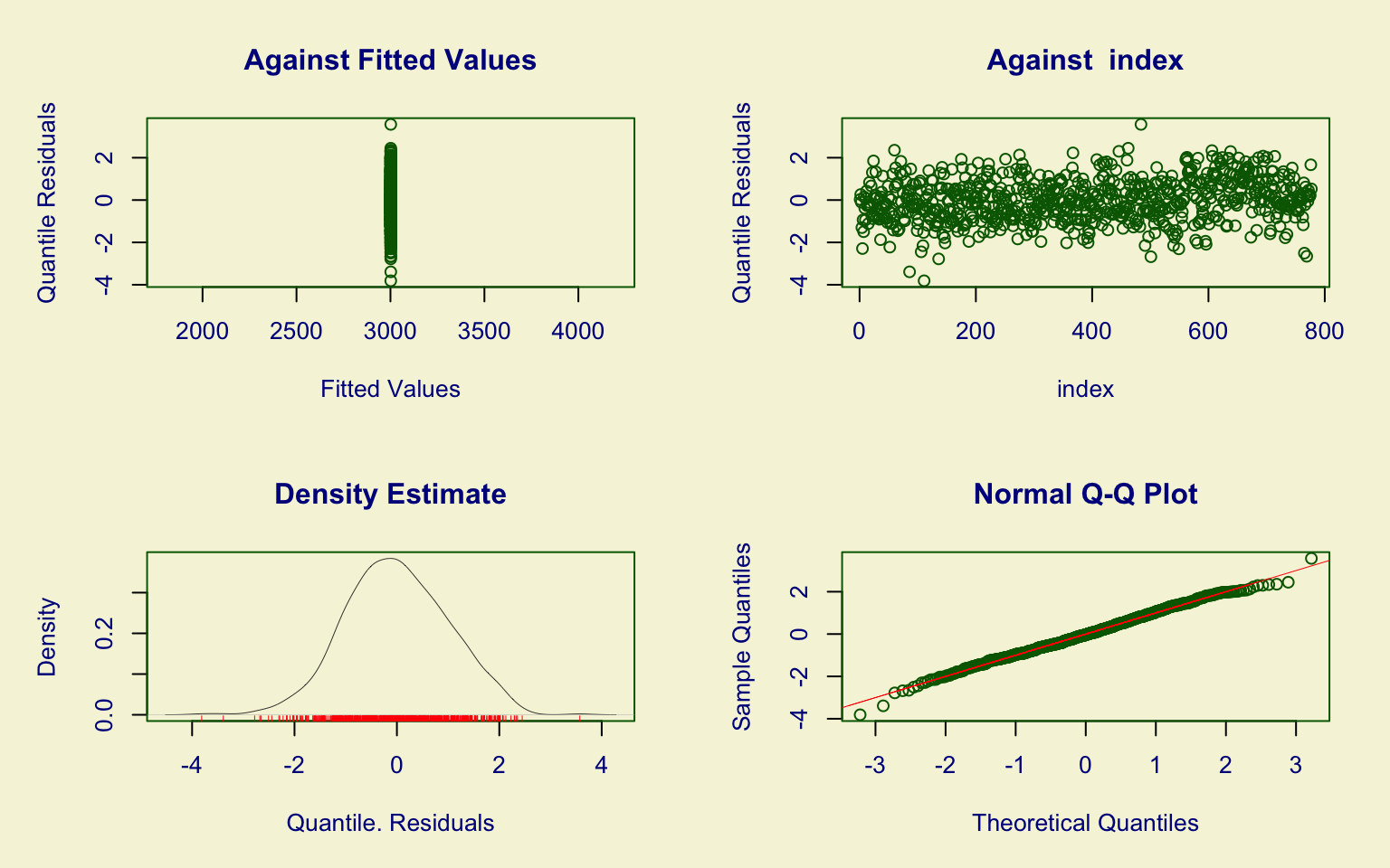
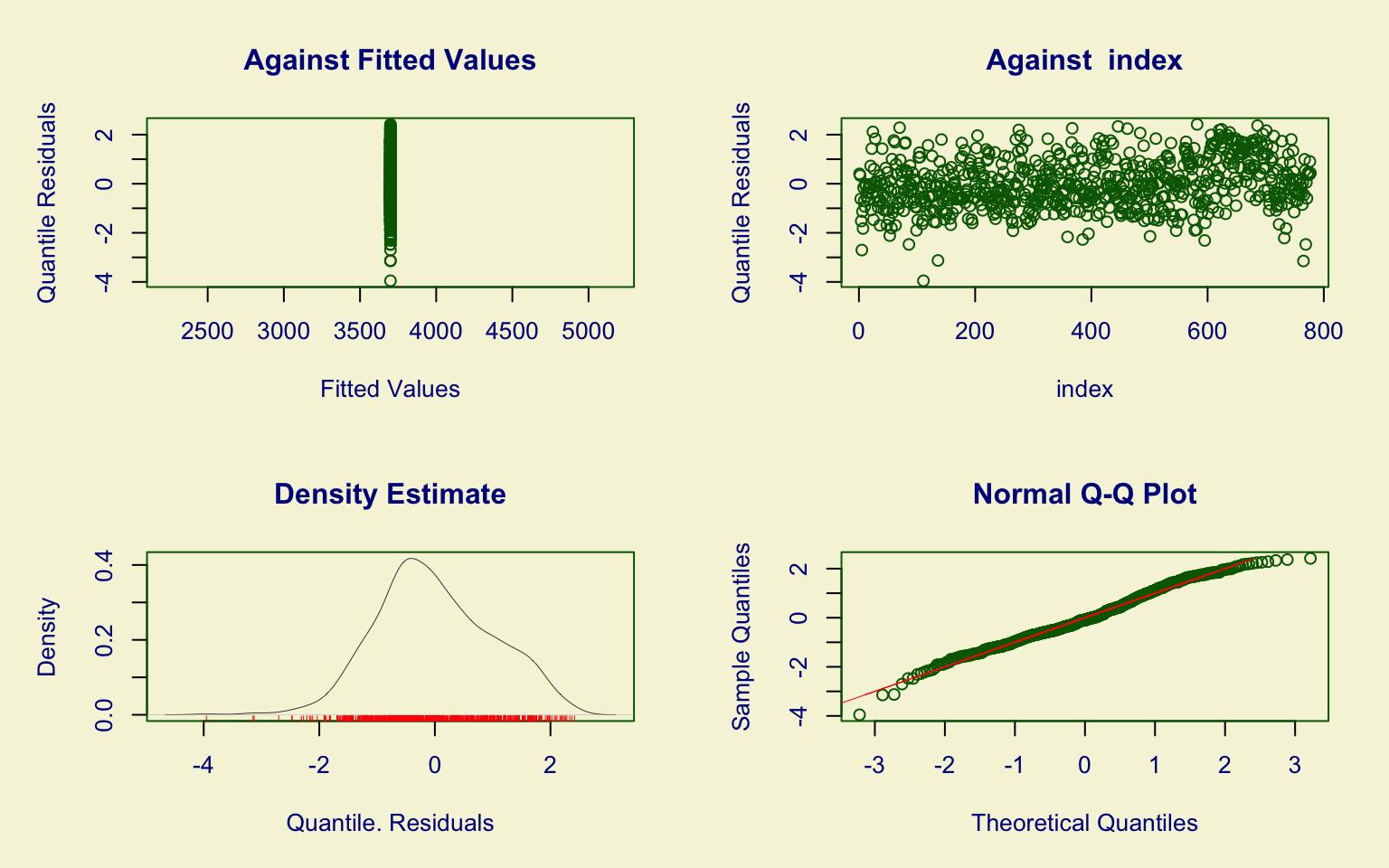
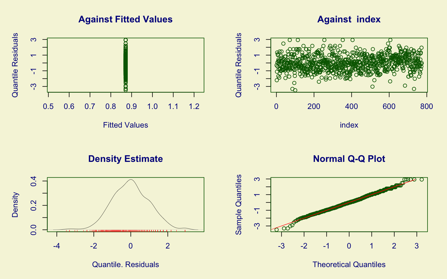
The residual diagnostic plots suggest an adequate fit:
- the Q-Q plot indicates a good alignment of the residuals with the theoretical normal distribution, with only minor deviations in the tails;
- the residual density is approximately symmetric and centered around zero.
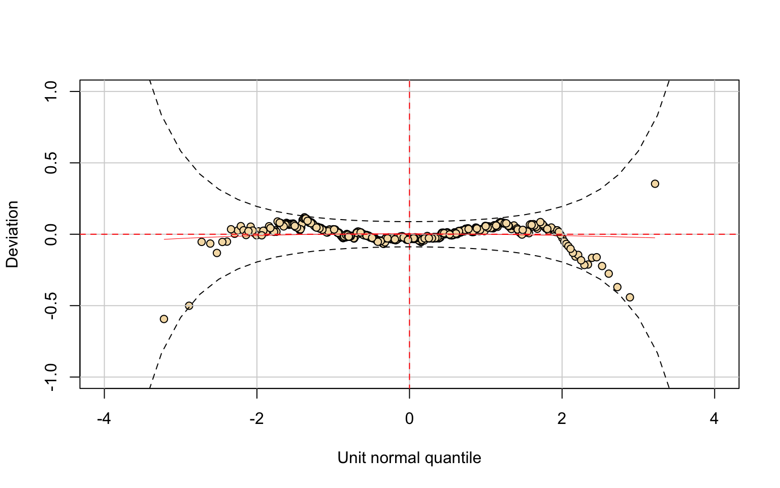
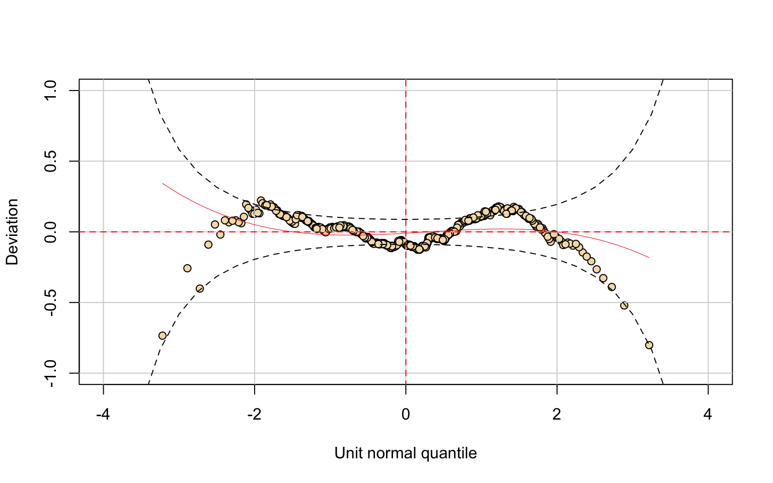
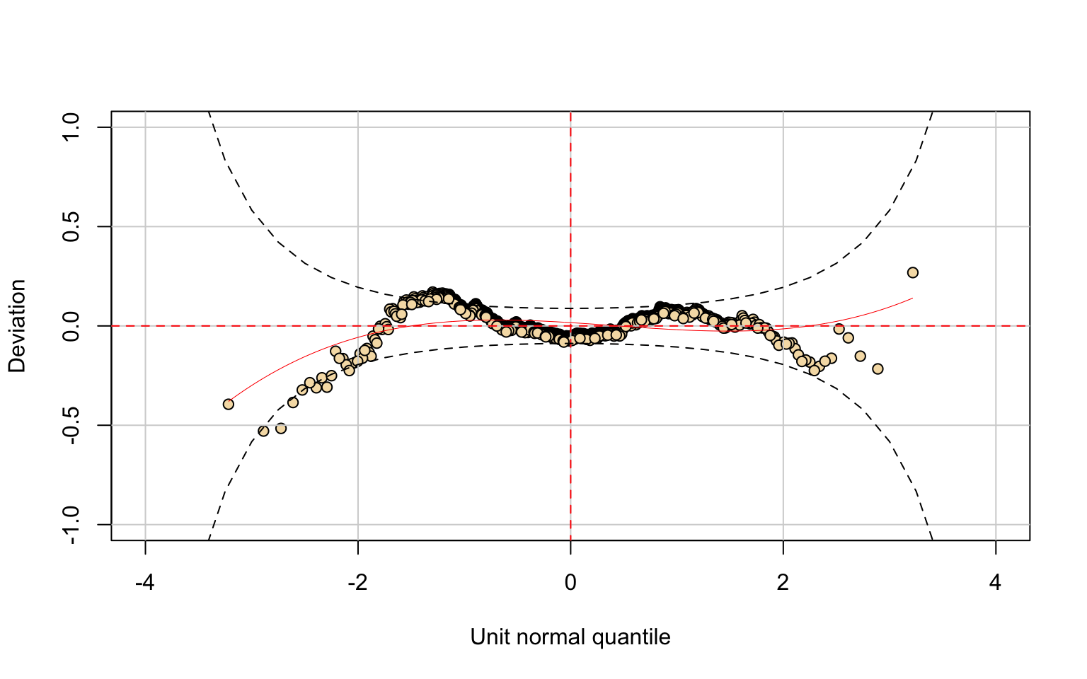
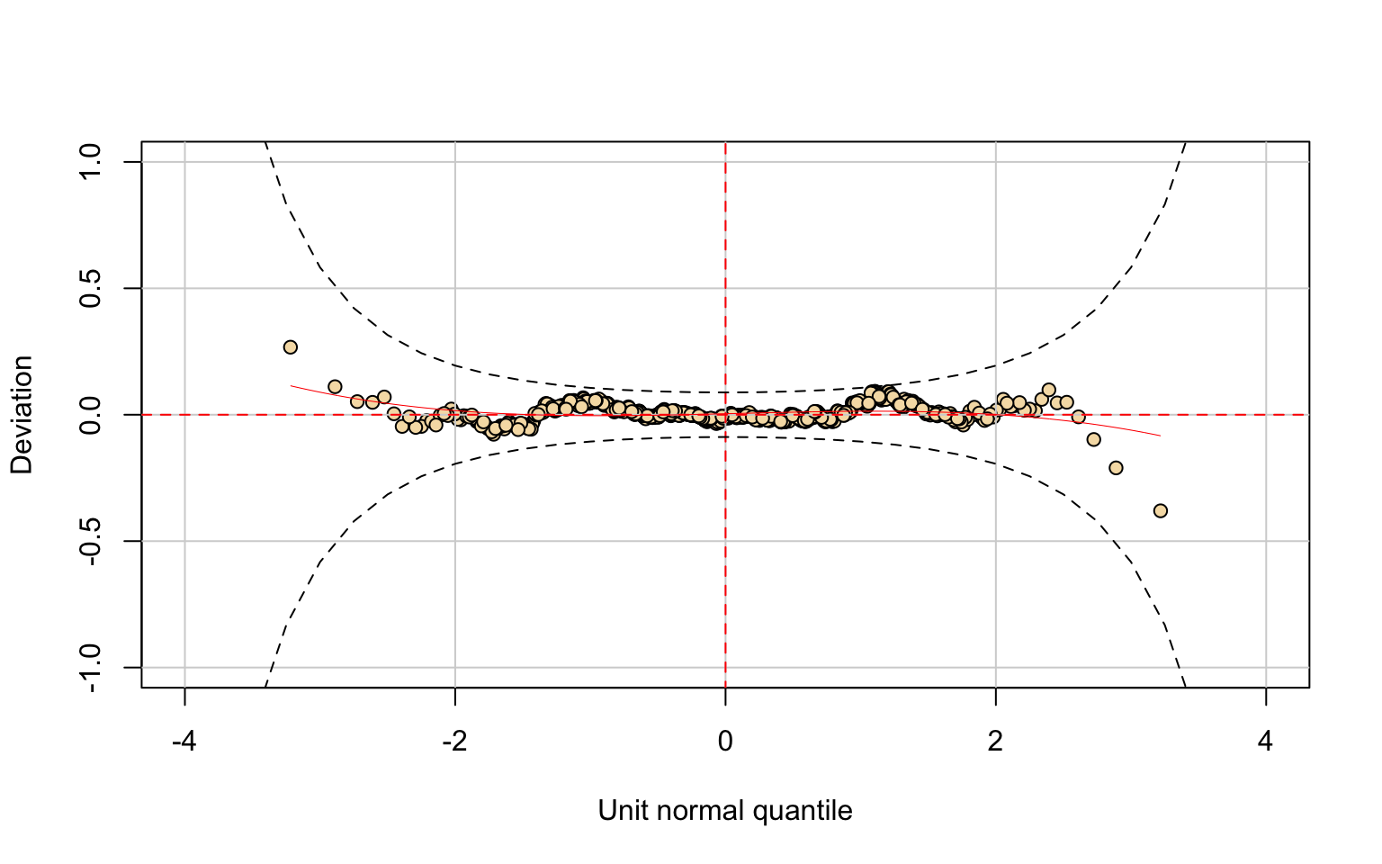
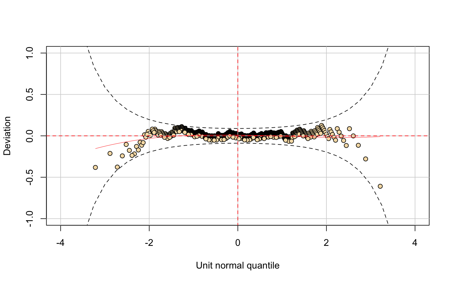
The worm plot supports these findings: most points lie within the confidence bands, with only mild systematic deviations in the tails. This indicates that the GIG model provides a satisfactory description of the data, although it may not perfectly capture the most extreme cases.
Finally, the Kolmogorov–Smirnov test (D = 0.0315, p-value = 0.4803) fails to reject the null hypothesis, further confirming the goodness of fit. Overall, the GIG distribution represents an appropriate choice to model the Applications variable.
Students accepted
Distribution Fitting
## *******************************************************************
## Family:  c("IG", "Inverse Gaussian")
##
## Call:  gamlssML(formula = y, family = DIST[i])
##
## Fitting method: "nlminb"
##
##
## Coefficient(s):
##             Estimate  Std. Error  t value   Pr(>|t|)
## eta.mu     7.6102623   0.0453237  167.909 < 2.22e-16 ***
## eta.sigma -3.5713367   0.0253673 -140.785 < 2.22e-16 ***
## ---
## Signif. codes:  0 '***' 0.001 '**' 0.01 '*' 0.05 '.' 0.1 ' ' 1
##
##  Degrees of Freedom for the fit: 2 Residual Deg. of Freedom   775
## Global Deviance:     13227.8
##             AIC:     13231.8
##             SBC:     13241.1
##
## Asymptotic one-sample Kolmogorov-Smirnov test
##
## data: unique(variable)
## D = 0.046259, p-value = 0.103
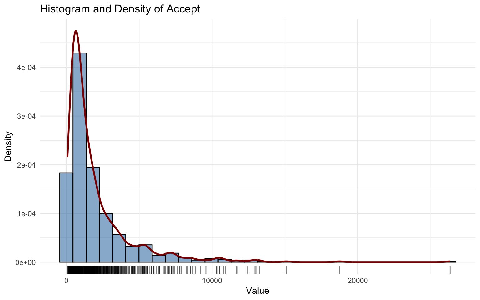
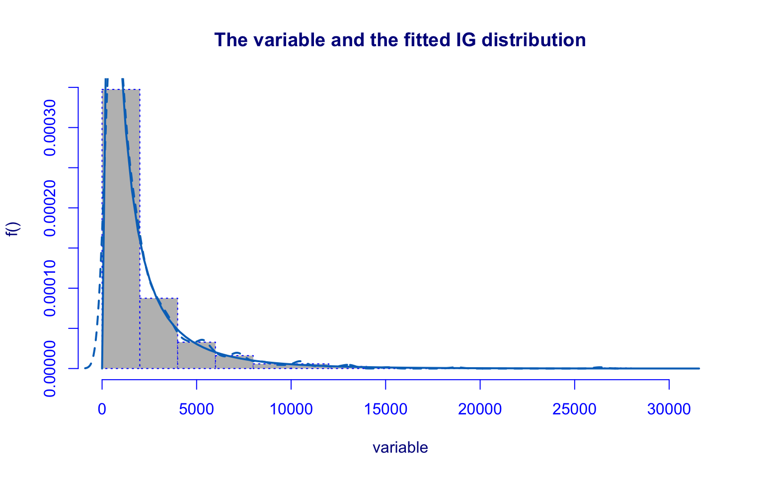
## alternative hypothesis: two-sidedThe Accept variable also shows a highly right-skewed distribution with several high-value outliers, similar to the Applications variable.
The distribution fitted using the Inverse Gaussian (IG) model works very well. This model has two parameters, \(\hat\mu\) and \(\hat\sigma\), and both are highly significant.
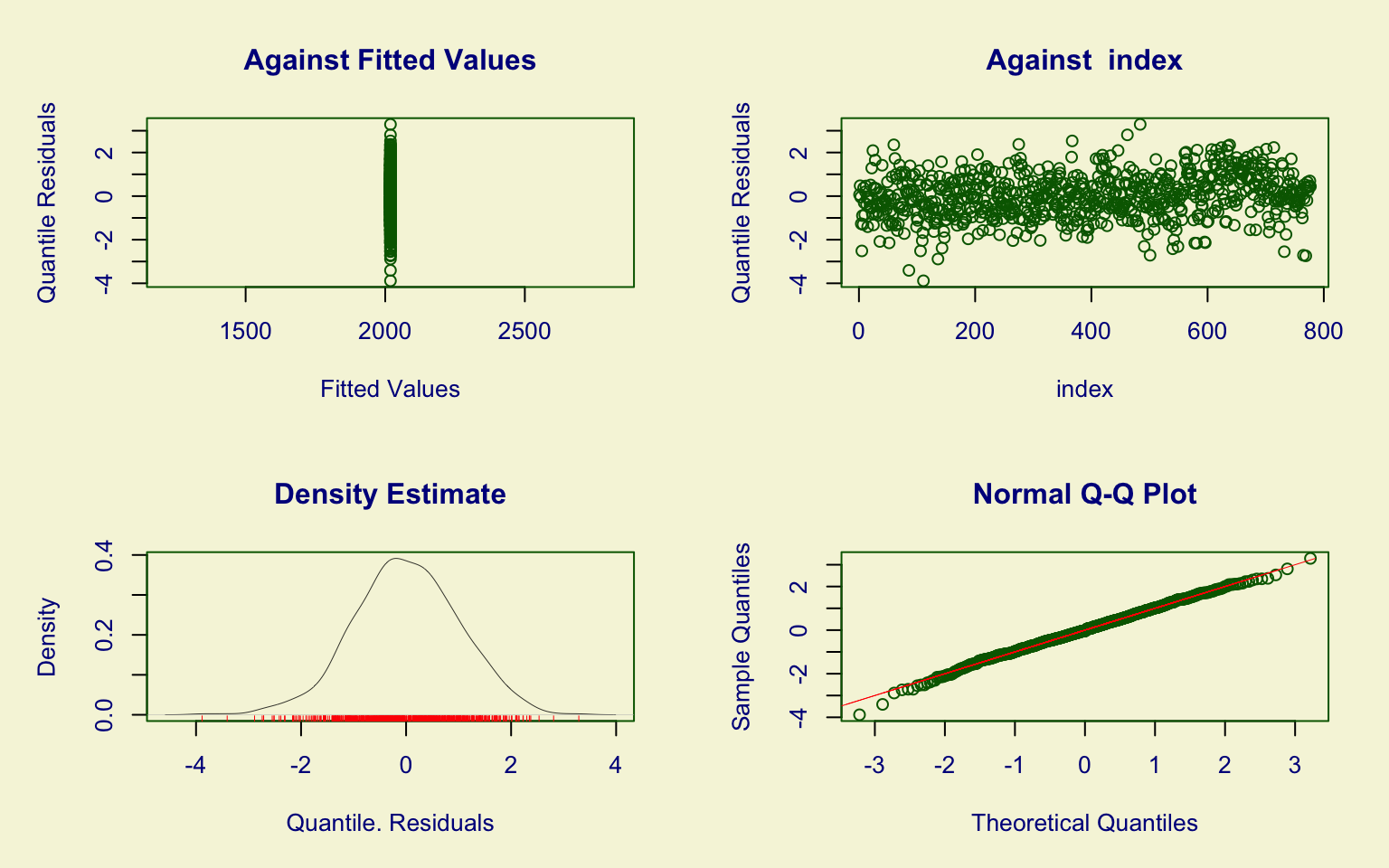
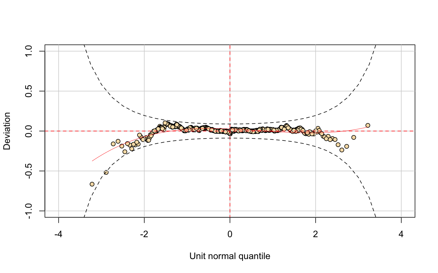
In the index plot, we can see that there is no dependency between rows (such as order effects). The quantile residuals are approximately distributed as \(\mathcal{N}(0,1),\) therefore the model fits very well.
The Kolmogorov–Smirnov test (D = 0.046259, p-value = 0.103) fails to reject the null hypothesis, further confirming the goodness of fit.
Hence, the IG distribution represents an appropriate choice for modeling the Accepted variable.
Students enrolled
Distribution Fitting
## *******************************************************************
## Family:  c("GIG", "Generalised Inverse Gaussian")
##
## Call:  gamlssML(formula = y, family = DIST[i])
##
## Fitting method: "nlminb"
##
##
## Coefficient(s):
##             Estimate  Std. Error   t value   Pr(>|t|)
## eta.mu     6.6592607   0.0463438 143.69245 < 2.22e-16 ***
## eta.sigma  0.2260256   0.0524799   4.30690 1.6556e-05 ***
## eta.nu    -0.7751681   0.1460976  -5.30582 1.1216e-07 ***
## ---
## Signif. codes:  0 '***' 0.001 '**' 0.01 '*' 0.05 '.' 0.1 ' ' 1
##
##  Degrees of Freedom for the fit: 3 Residual Deg. of Freedom   774
## Global Deviance:     11691.3
##             AIC:     11697.3
##             SBC:     11711.3
##
## Asymptotic one-sample Kolmogorov-Smirnov test
##
## data: unique(variable)
## D = 0.081749, p-value = 0.0008482
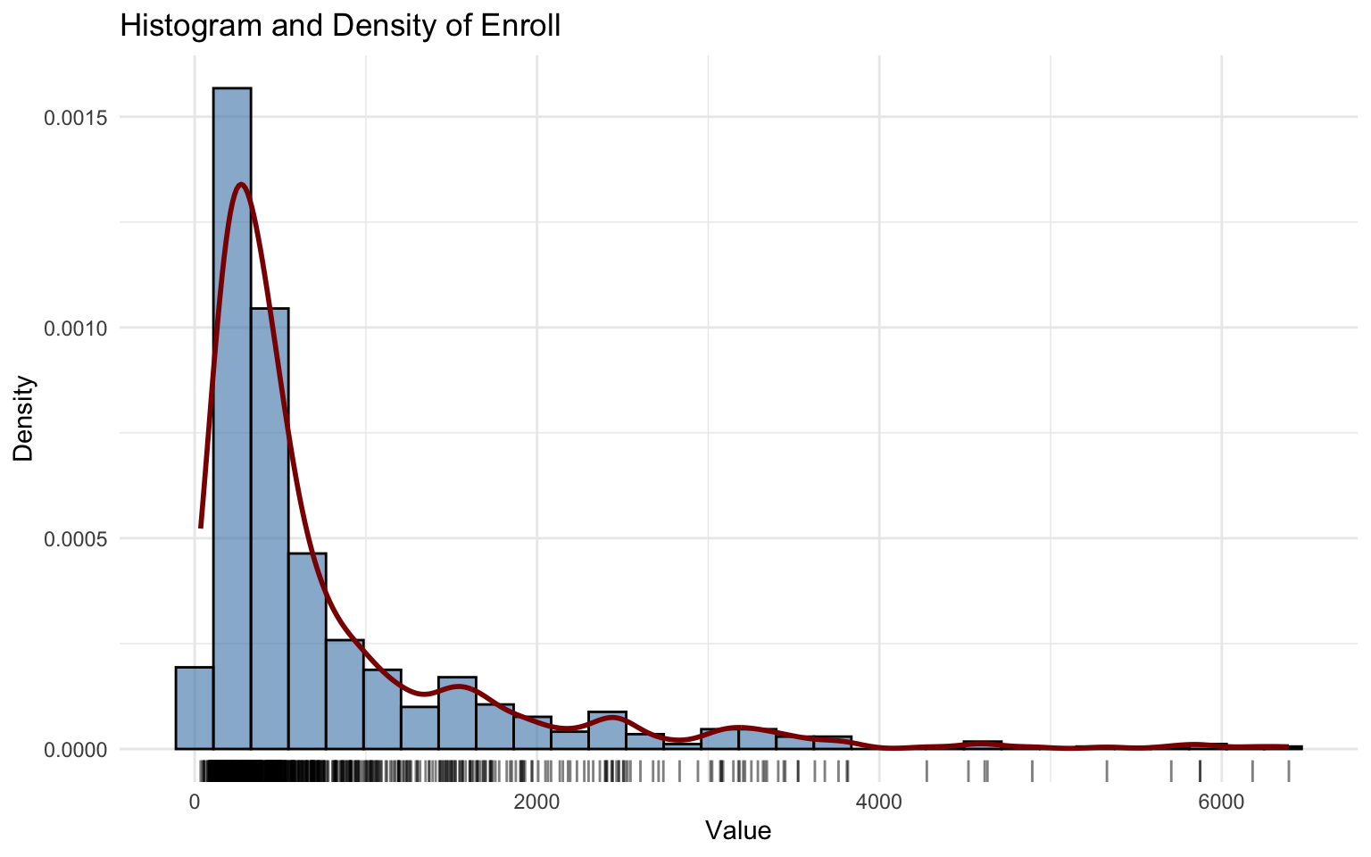
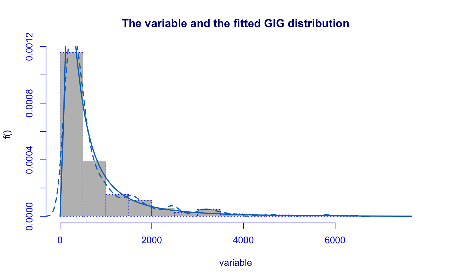
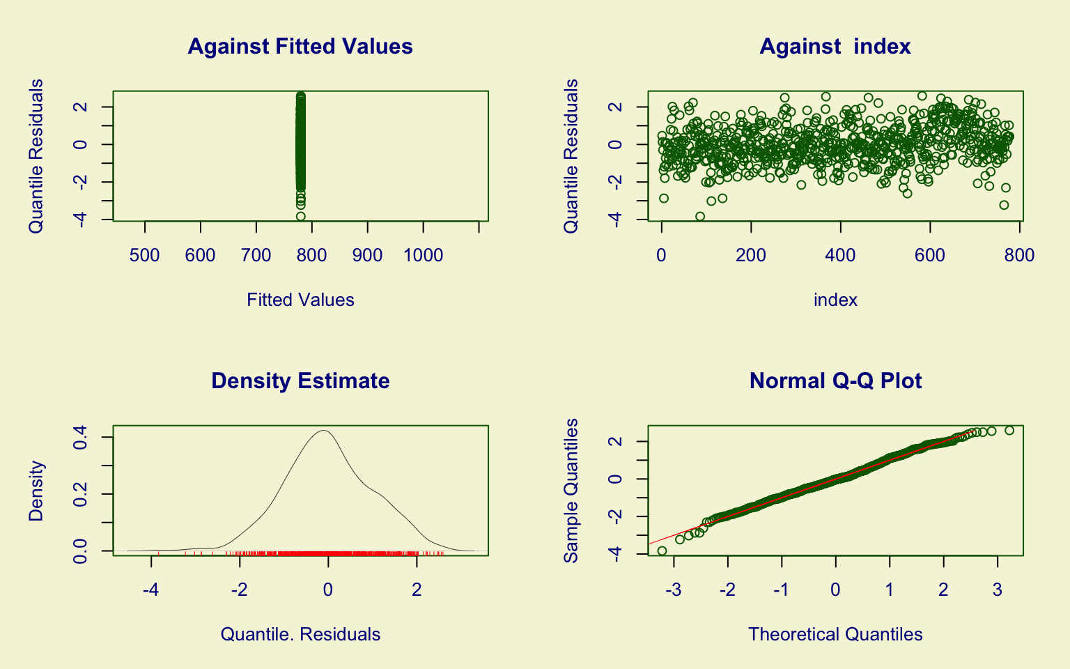
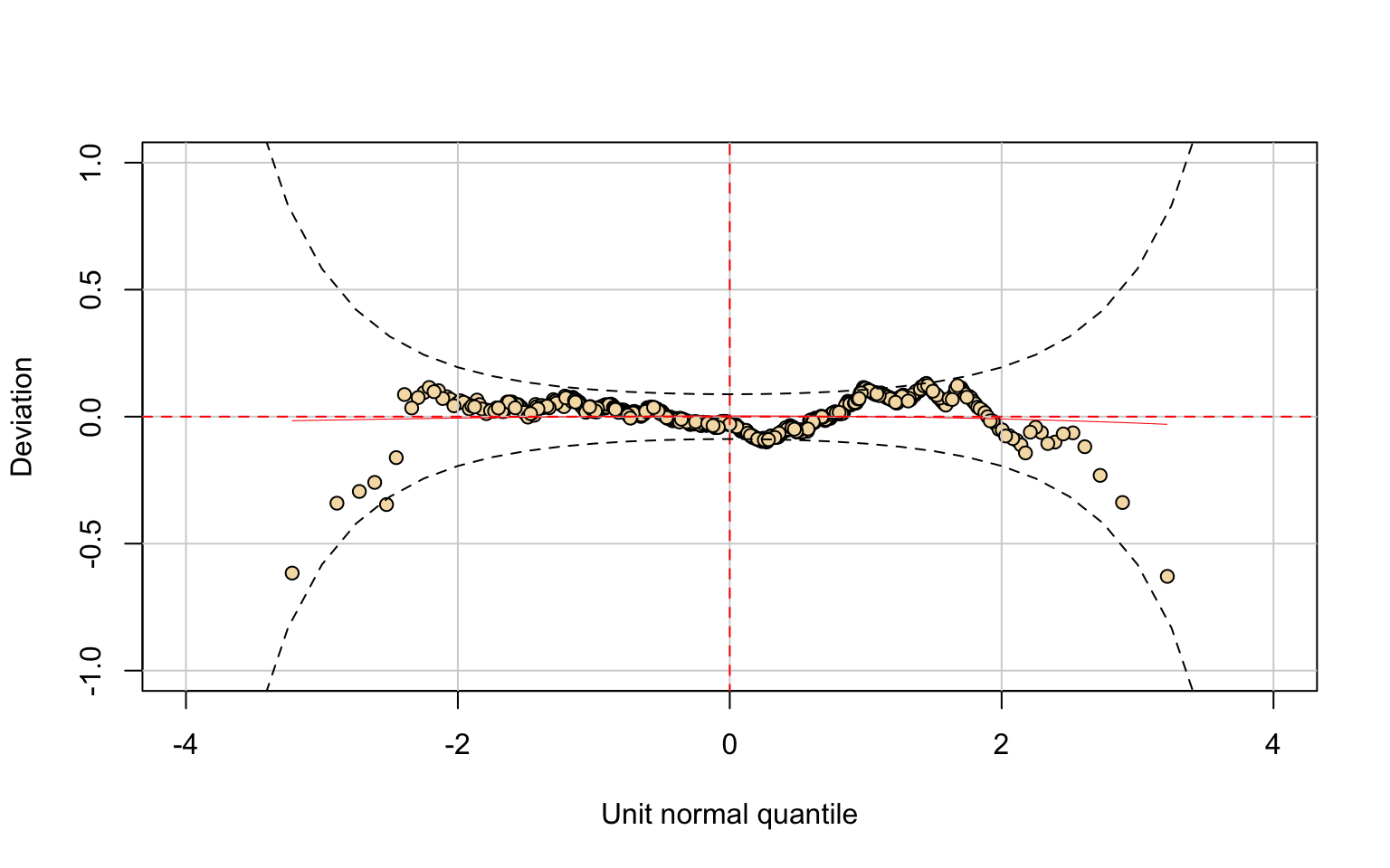
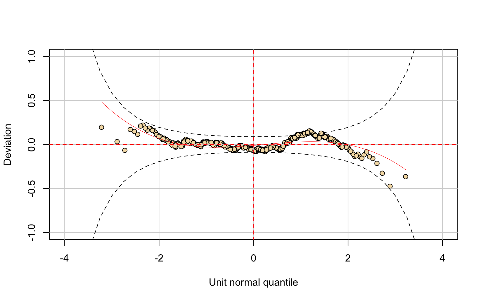
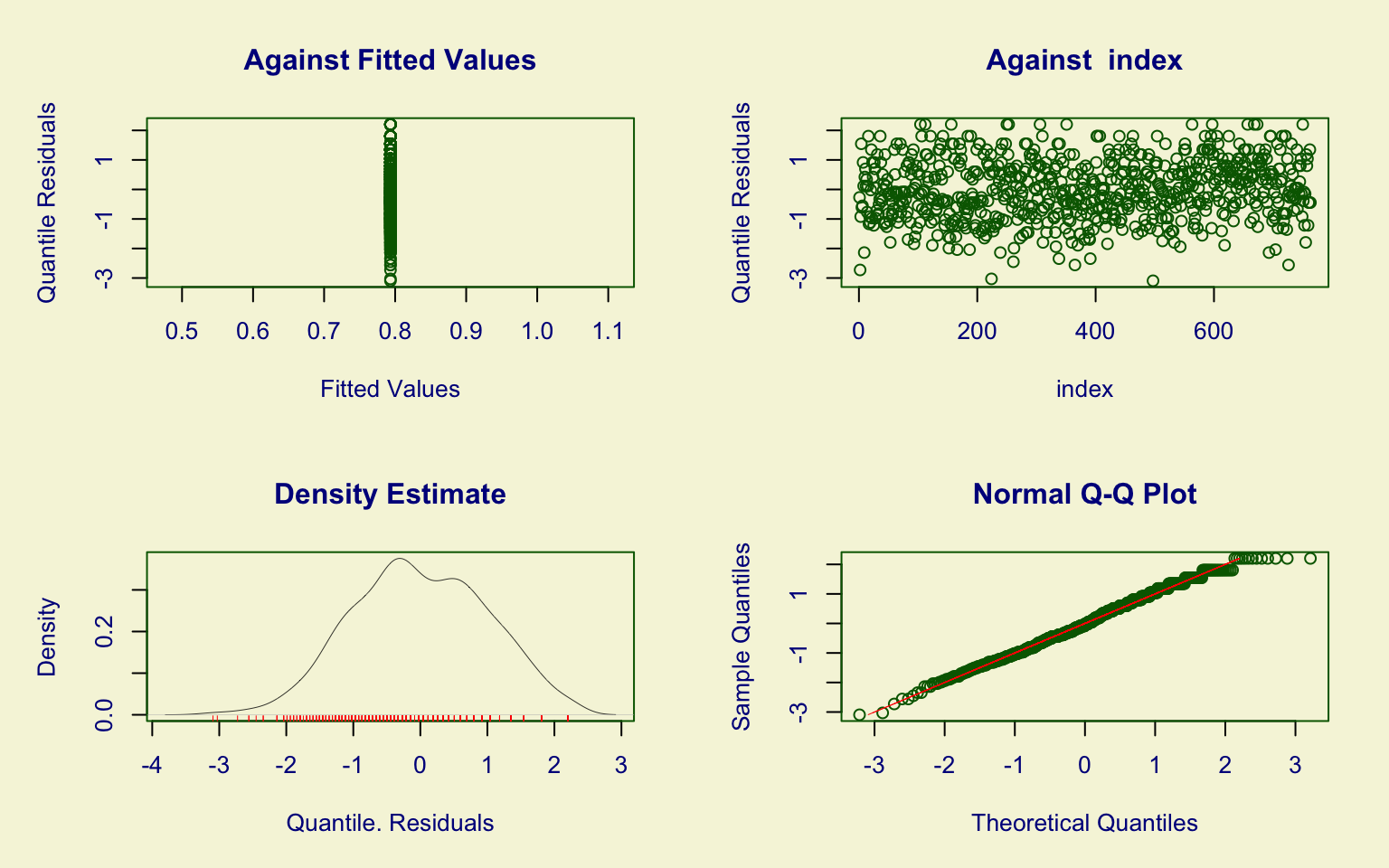
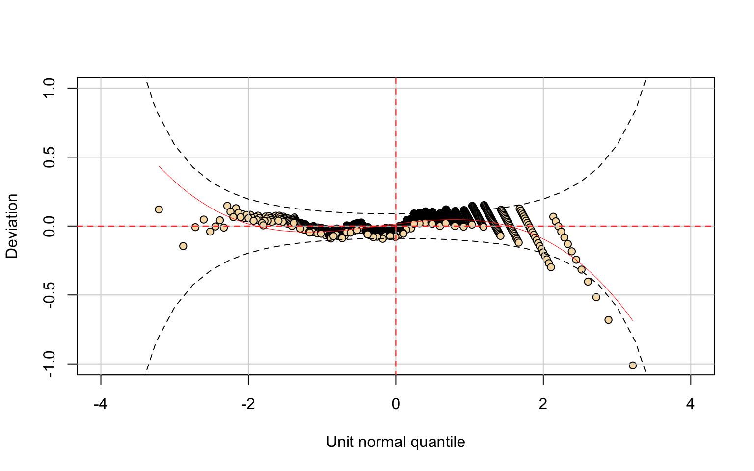
## alternative hypothesis: two-sidedThe Enroll variable also shows a highly right-skewed distribution with several high-value outliers. However, in this case, there is a slight increase just before the value 2000, so the distribution is not monotonically decreasing.
Even though the parameter estimates are significant, the Generalised Inverse Gaussian (GIG) model does not capture this small increase. This can be seen in the residual density plot (which is not symmetric) and in the worm plot (where some normal quantiles are very close to the 95% confidence interval).
The Kolmogorov–Smirnov test (D = 0.081749, p-value = 0.0008482) rejects the null hypothesis.
Hence, the GIG model fits well for values below 1000, but for values greater than 1000 the fit is less accurate.
Top 10%
Distribution Fitting
## *******************************************************************
## Family:  c("GB1", "Generalized beta type 1")
##
## Call:  gamlssML(formula = y, family = DIST[i])
##
## Fitting method: "nlminb"
##
##
## Coefficient(s):
##            Estimate  Std. Error  t value   Pr(>|t|)
## eta.mu    -0.161851    0.136263 -1.18778  0.2349190
## eta.sigma  0.454322    0.149667  3.03556  0.0024009 **
## eta.nu    -4.016184    0.611128 -6.57176 4.9724e-11 ***
## eta.tau    1.077745    0.156445  6.88895 5.6206e-12 ***
## ---
## Signif. codes:  0 '***' 0.001 '**' 0.01 '*' 0.05 '.' 0.1 ' ' 1
##
##  Degrees of Freedom for the fit: 4 Residual Deg. of Freedom   773
## Global Deviance:     -789.978
##             AIC:     -781.978
##             SBC:     -763.356
##
## Exact one-sample Kolmogorov-Smirnov test
##
## data: unique(variable)
## D = 0.33988, p-value = 5.886e-09
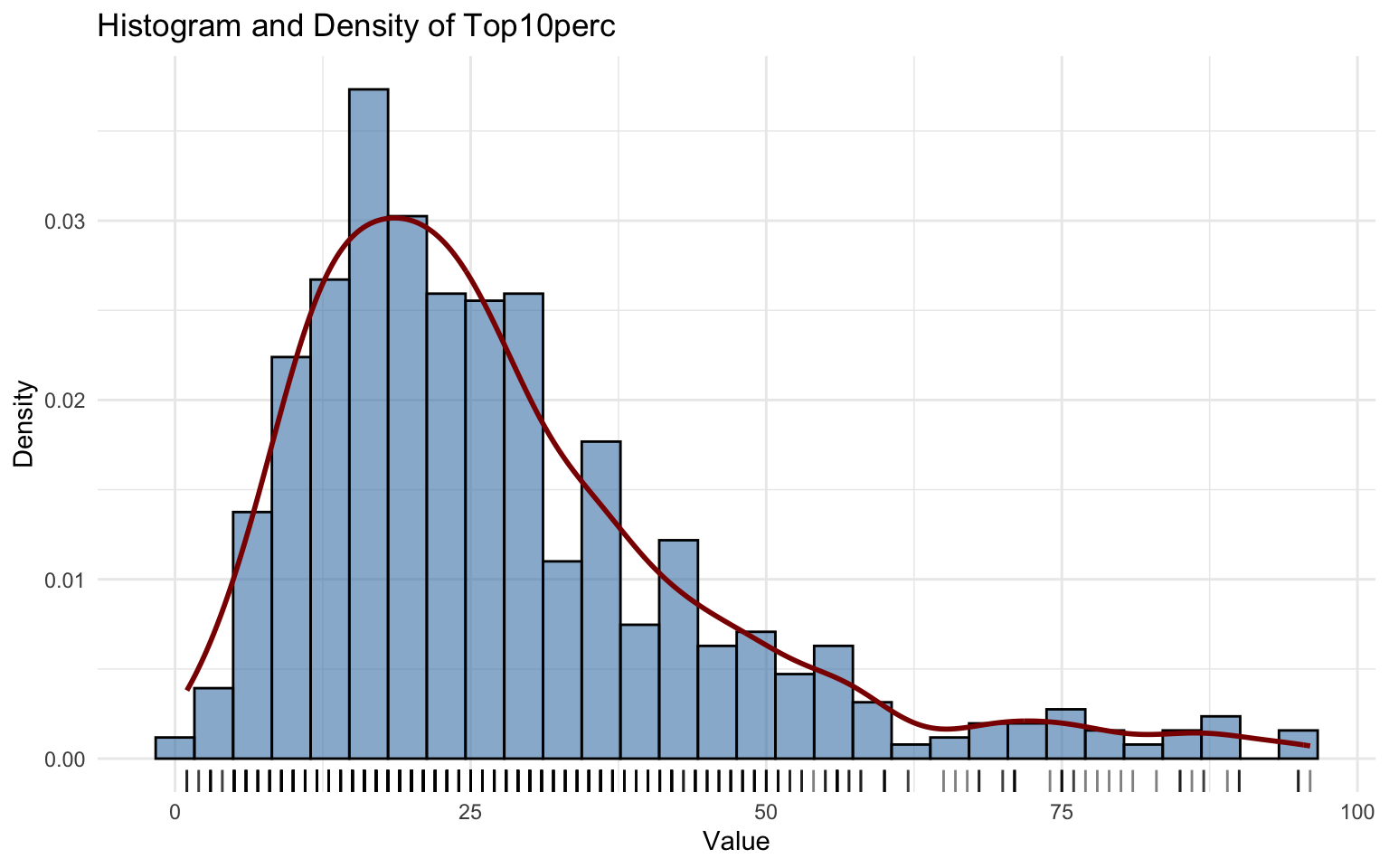
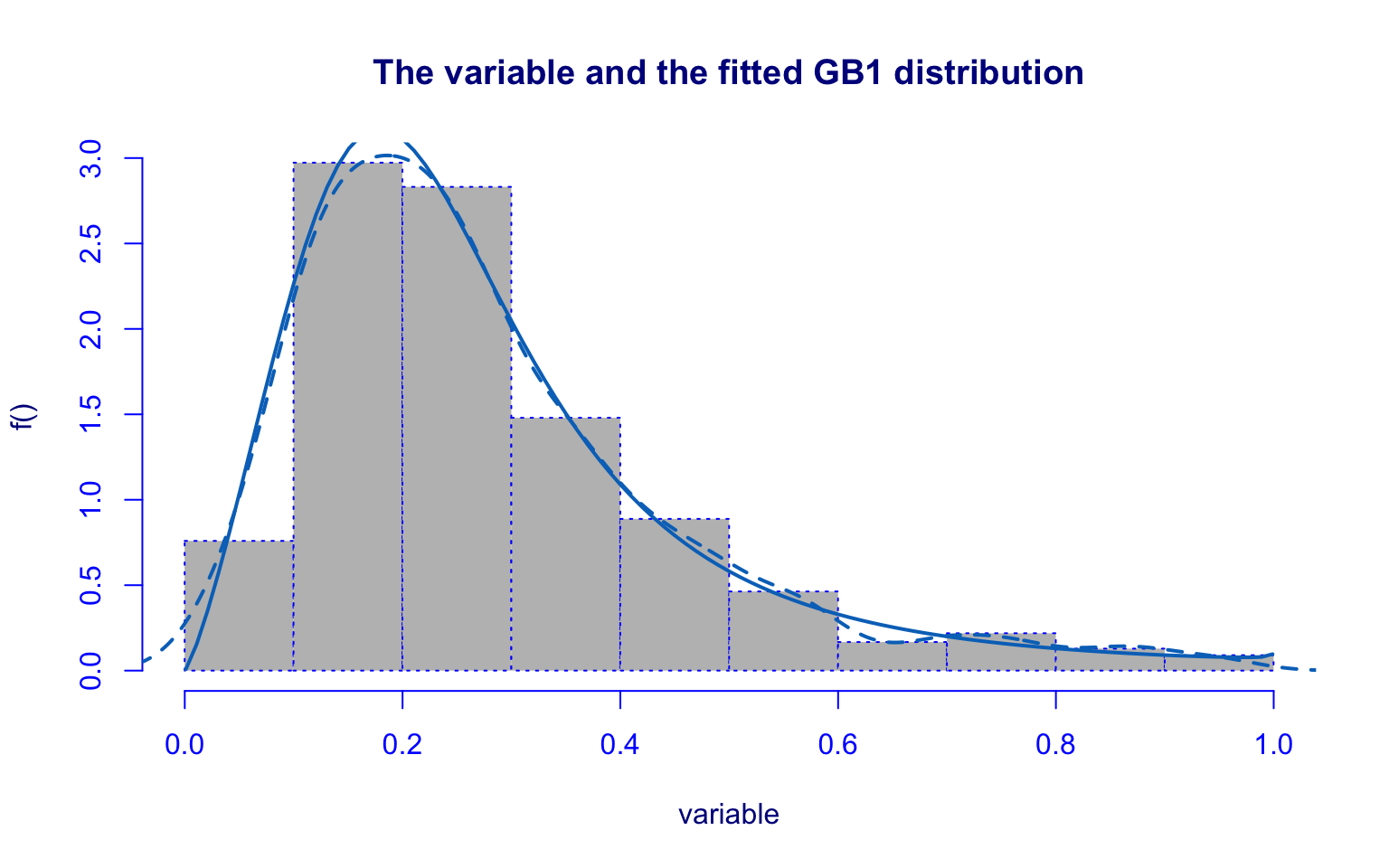
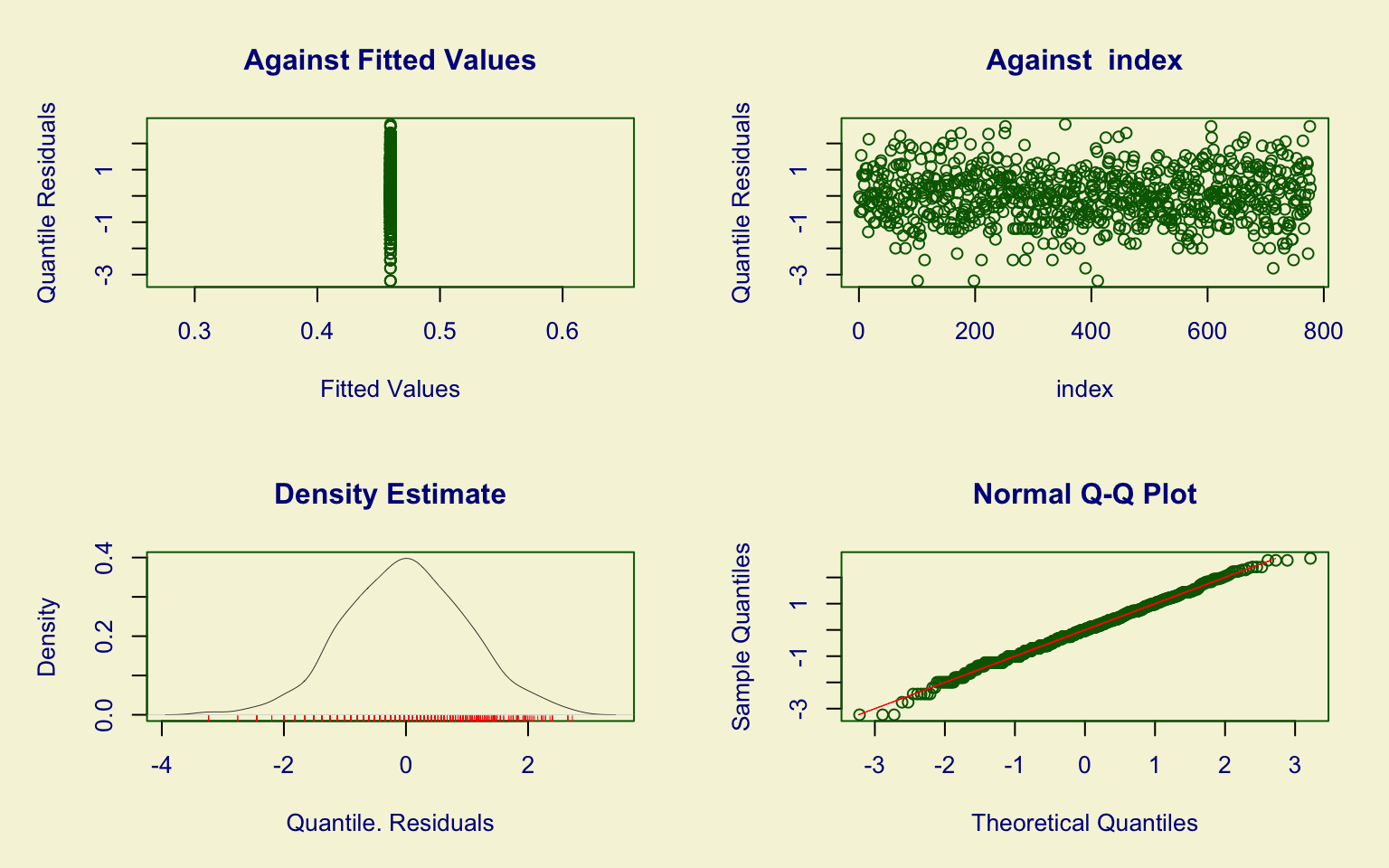
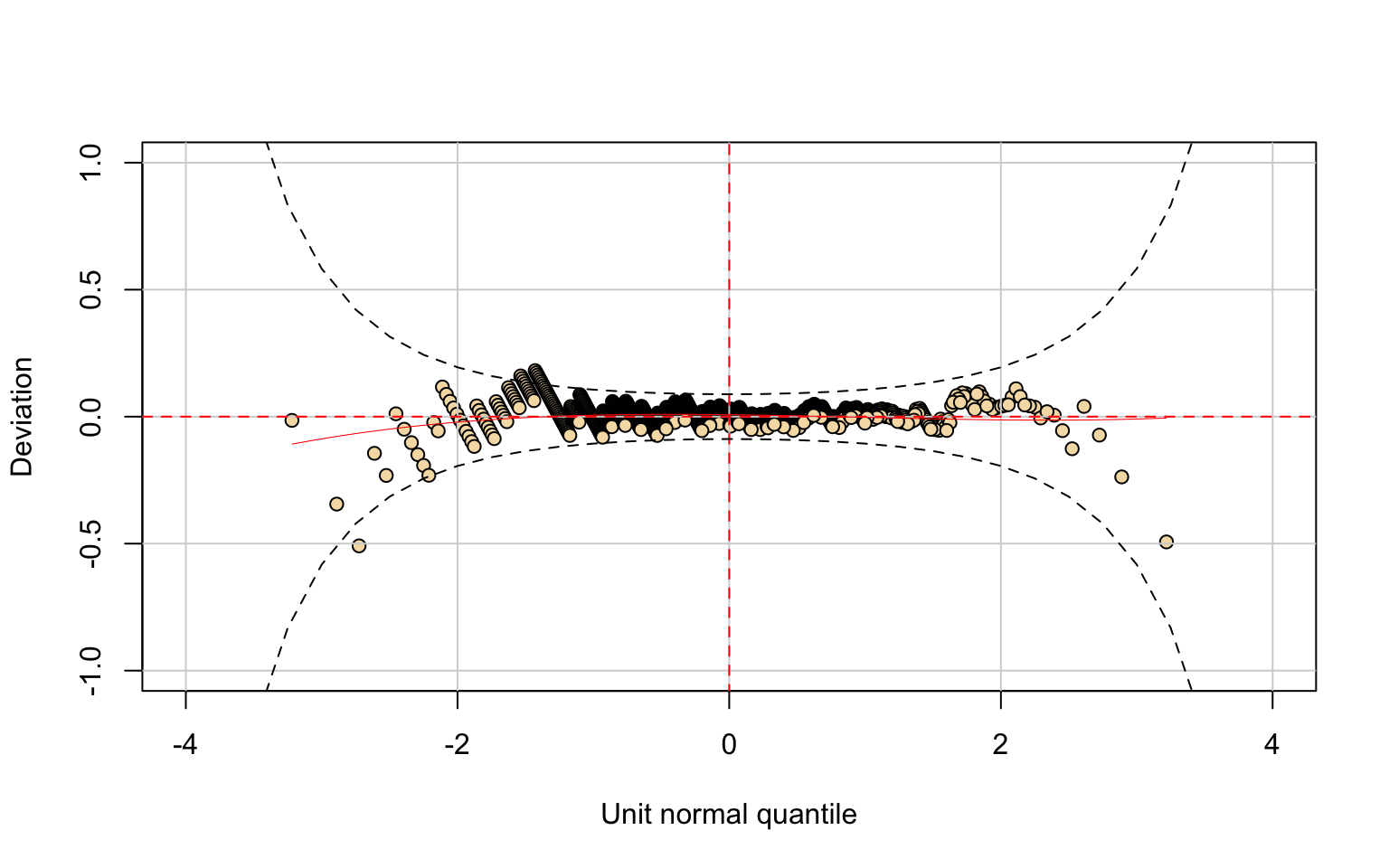
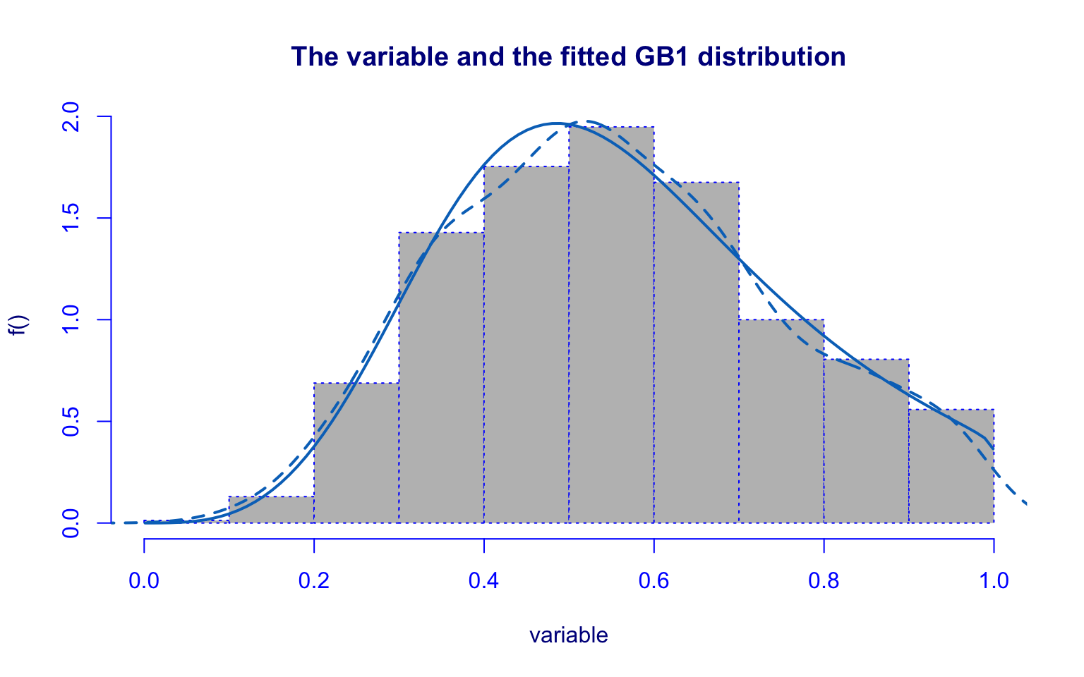
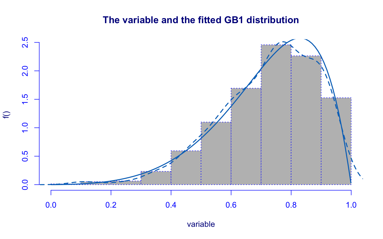
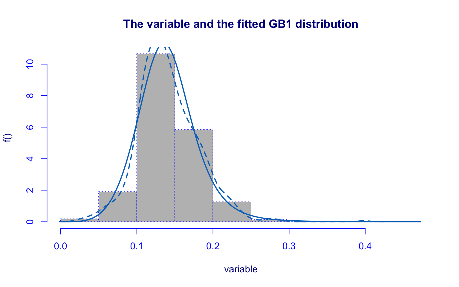
## alternative hypothesis: two-sidedThe Top10perc variable is highly right-skewed, with some outliers above 65%.
The fitted distribution is the Generalized Beta type 1 (GB1). Most parameters are significant, with the exception of \(\hat\mu\).
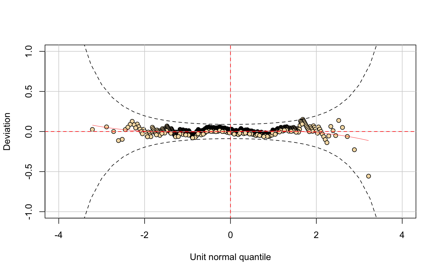
Diagnostic checks highlight several issues:
- the worm plot shows points outside the 95% confidence bands;
- the residual density is asymmetric;
- the Kolmogorov–Smirnov test (D = 0.33988, p-value = 5.886e-09) rejects the null hypothesis.
Hence, the GB1 model does not adequately capture the distribution of this variable.
Top 25%
Distribution Fitting

## *******************************************************************
## Family:  c("GB1", "Generalized beta type 1")
##
## Call:  gamlssML(formula = y, family = DIST[i])
##
## Fitting method: "nlminb"
##
##
## Coefficient(s):
##            Estimate  Std. Error  t value   Pr(>|t|)
## eta.mu     0.194144    0.289582  0.67043    0.50258
## eta.sigma  0.200006    0.192980  1.03641    0.30001
## eta.nu    -2.153256    0.313620 -6.86582 6.6112e-12 ***
## eta.tau    1.190385    0.235046  5.06448 4.0952e-07 ***
## ---
## Signif. codes:  0 '***' 0.001 '**' 0.01 '*' 0.05 '.' 0.1 ' ' 1
##
##  Degrees of Freedom for the fit: 4 Residual Deg. of Freedom   766
## Global Deviance:     -400.959
##             AIC:     -392.959
##             SBC:     -374.373
##
## Exact one-sample Kolmogorov-Smirnov test
##
## data: unique(variable)
## D = 0.12648, p-value = 0.1097
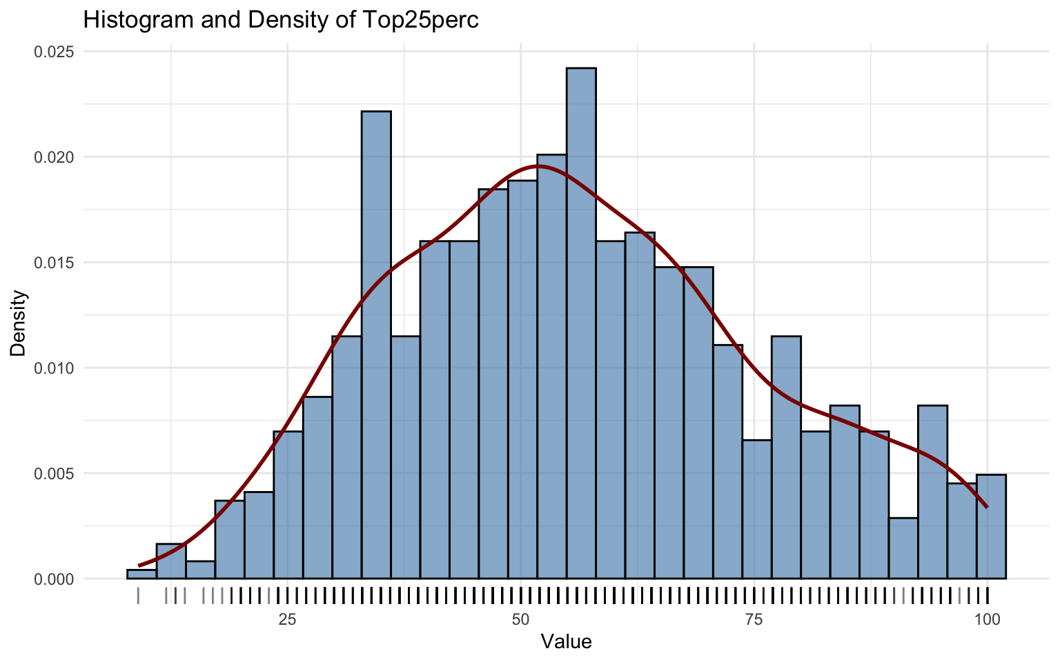
## alternative hypothesis: two-sidedThe Top25perc distribution is more symmetric compared to Top10perc, although similar issues remain.
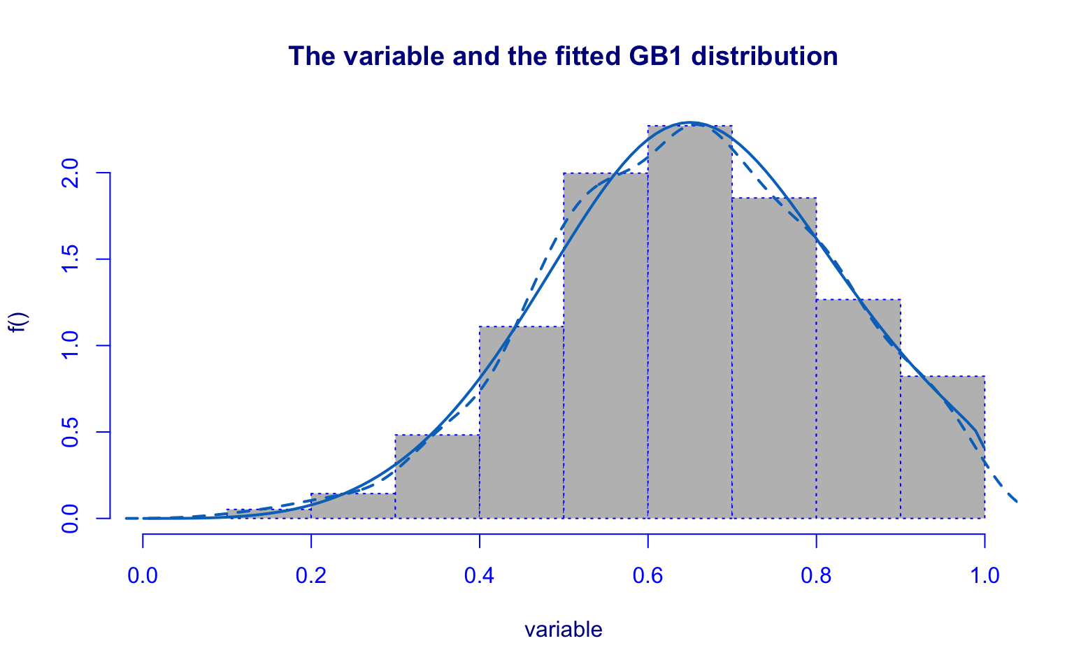
In this case, the Generalized Beta type 1 (GB1) distribution again provides the best fit. However, the parameter \(\hat\sigma\) is not significant.
From a graphical perspective, the residuals behave better than in Top10perc, and the Kolmogorov–Smirnov test fails to reject the null hypothesis, suggesting an acceptable overall fit despite some limitations.
Full-time undergraduates
Distribution Fitting
## *******************************************************************
## Family:  c("GIG", "Generalised Inverse Gaussian")
##
## Call:  gamlssML(formula = y, family = DIST[i])
##
## Fitting method: "nlminb"
##
##
## Coefficient(s):
##             Estimate  Std. Error   t value   Pr(>|t|)
## eta.mu     8.2160631   0.0561717 146.26697 < 2.22e-16 ***
## eta.sigma  0.3946007   0.0716927   5.50405 3.7115e-08 ***
## eta.nu    -0.9077921   0.1186020  -7.65410 1.9540e-14 ***
## ---
## Signif. codes:  0 '***' 0.001 '**' 0.01 '*' 0.05 '.' 0.1 ' ' 1
##
##  Degrees of Freedom for the fit: 3 Residual Deg. of Freedom   774
## Global Deviance:     14046.7
##             AIC:     14052.7
##             SBC:     14066.7
##
## Asymptotic one-sample Kolmogorov-Smirnov test
##
## data: unique(variable)
## D = 0.044836, p-value = 0.1133
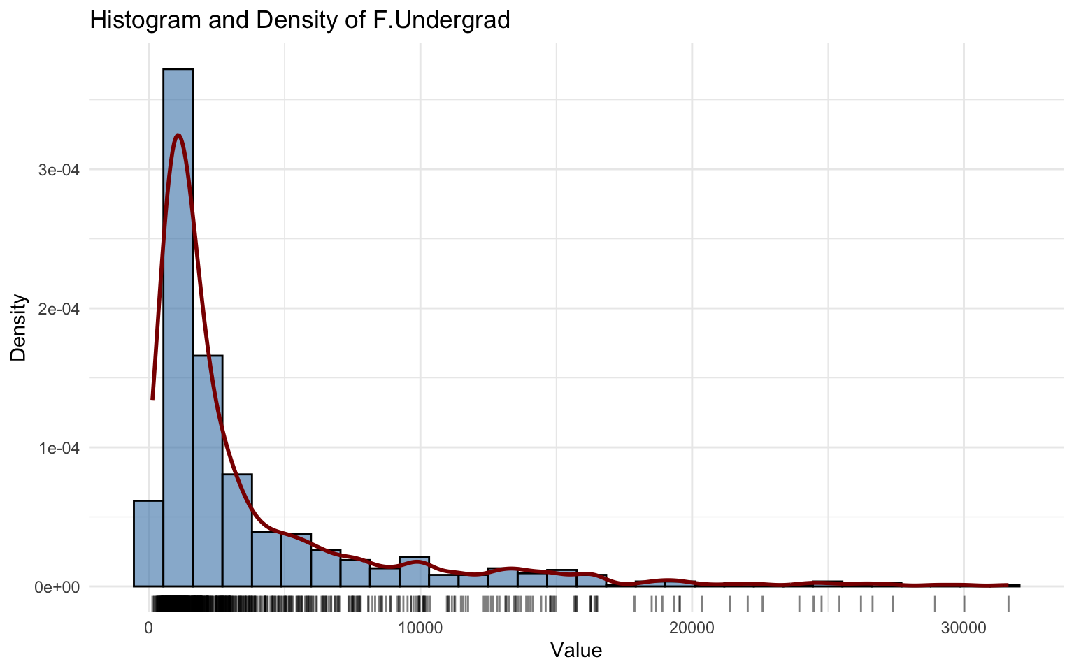
## alternative hypothesis: two-sidedThe F.Undergrad variable is highly right-skewed with several large outliers.
The Generalized Inverse Gaussian (GIG) model fits well, with all three parameters \(\hat\mu, \hat\sigma, \hat\nu\) highly significant.
Residual diagnostics show:
- quantile residuals approximately distributed as \(N(0,1)\), with some fluctuations;
- the worm plot indicates heavier tails (S-shaped curve), suggesting excess kurtosis.
The Kolmogorov–Smirnov test (D = 0.044836, p-value = 0.1133) fails to reject the null hypothesis, supporting a satisfactory fit, though not perfect in the tails.
Part-time undergraduates
Distribution Fitting
## *******************************************************************
## Family:  c("BCPEo", "Box-Cox Power Exponential-orig.")
##
## Call:  gamlssML(formula = y, family = DIST[i])
##
## Fitting method: "nlminb"
##
##
## Coefficient(s):
##            Estimate  Std. Error  t value   Pr(>|t|)
## eta.mu    5.8169964   0.0635828 91.48690 < 2.22e-16 ***
## eta.sigma 0.4616539   0.0245371 18.81456 < 2.22e-16 ***
## eta.nu    0.1008651   0.0173222  5.82287 5.7845e-09 ***
## eta.tau   0.8734533   0.0806019 10.83663 < 2.22e-16 ***
## ---
## Signif. codes:  0 '***' 0.001 '**' 0.01 '*' 0.05 '.' 0.1 ' ' 1
##
##  Degrees of Freedom for the fit: 4 Residual Deg. of Freedom   773
## Global Deviance:     11782
##             AIC:     11790
##             SBC:     11808.6
##
## Asymptotic one-sample Kolmogorov-Smirnov test
##
## data: unique(variable)
## D = 0.14887, p-value = 2.545e-11
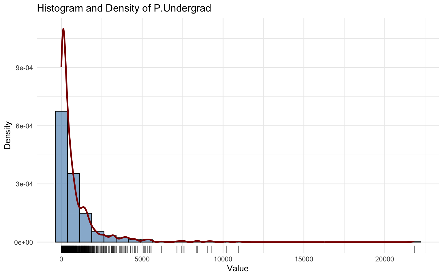
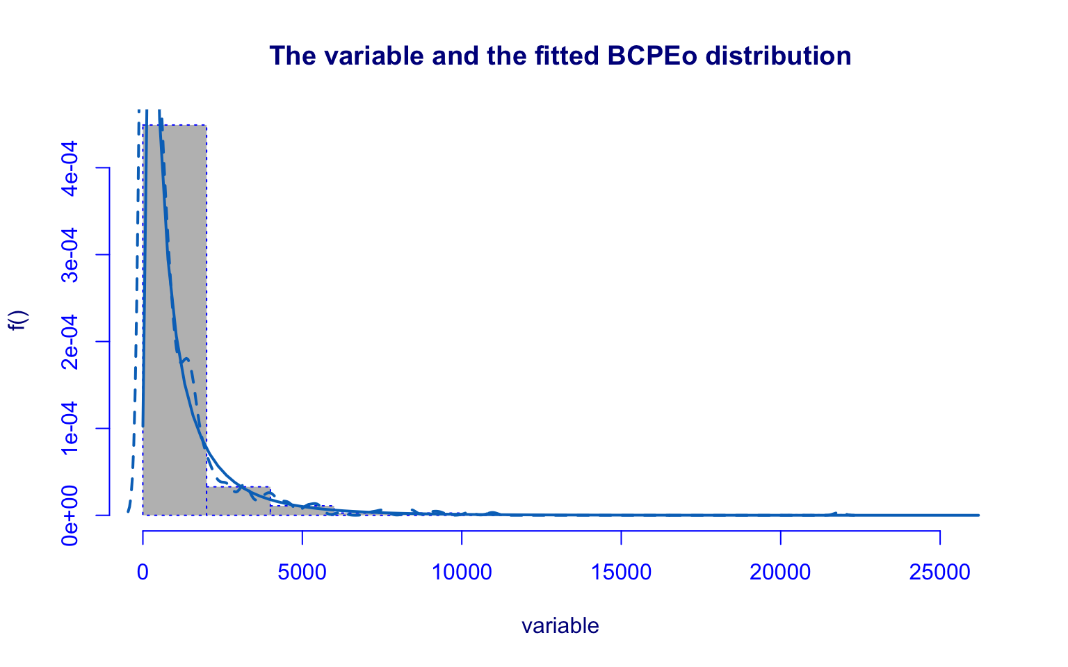
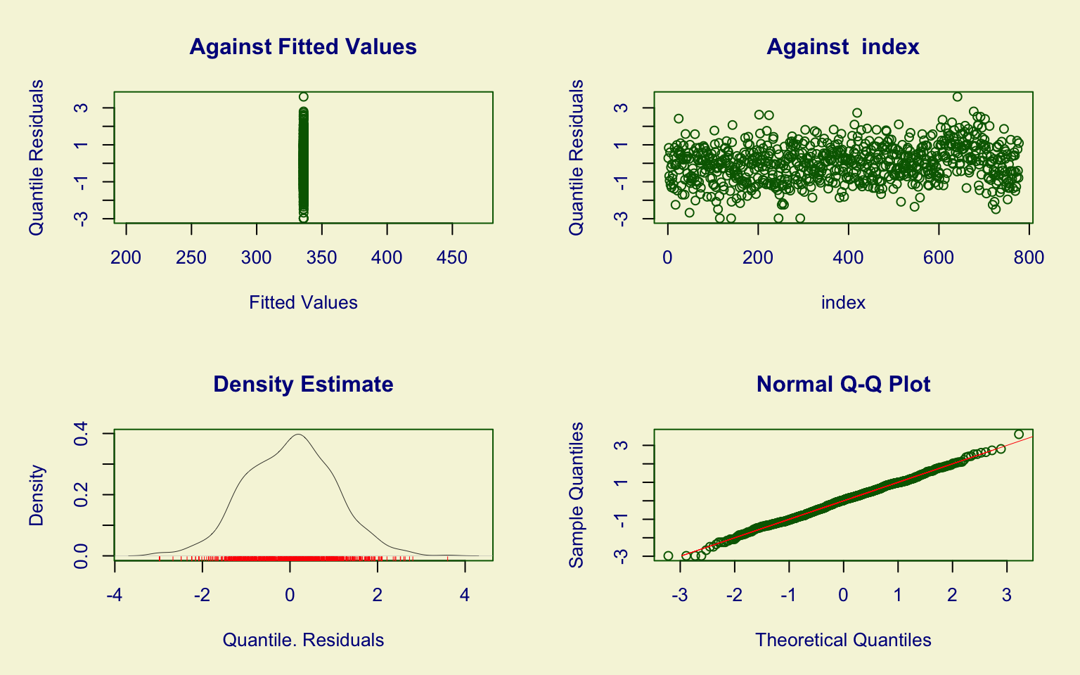
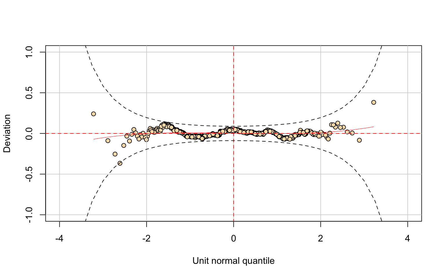
## alternative hypothesis: two-sidedThe P.Undergrad variable is extremely concentrated near zero and highly right-skewed with large outliers.
The selected model is the Box-Cox Power Exponential-original (BCPEo). All parameters \(\theta = (\hat\mu, \hat\sigma, \hat\nu, \hat\tau)\) are significant.
However, diagnostic checks reveal problems:
- the residual density is asymmetric;
- the Kolmogorov–Smirnov test (D = 0.14887, p-value = 2.545e-11) rejects the null hypothesis.
Thus, despite parameter significance, the BCPEo distribution does not provide an adequate fit.
Out-of-state tuition
Distribution Fitting
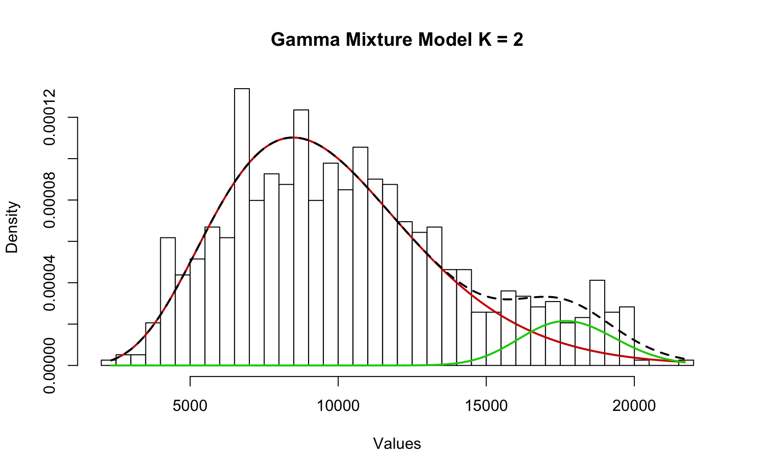
## Gamma mixture model with 2 components
## comp1 comp2
## pi 0.9126484 8.735160e-02
## mu 9732.5083079 1.783953e+04
## sd 3496.9897502 1.628513e+03
## shape 7.7457031 1.200008e+02
## rate 0.0007959 6.726700e-03
##
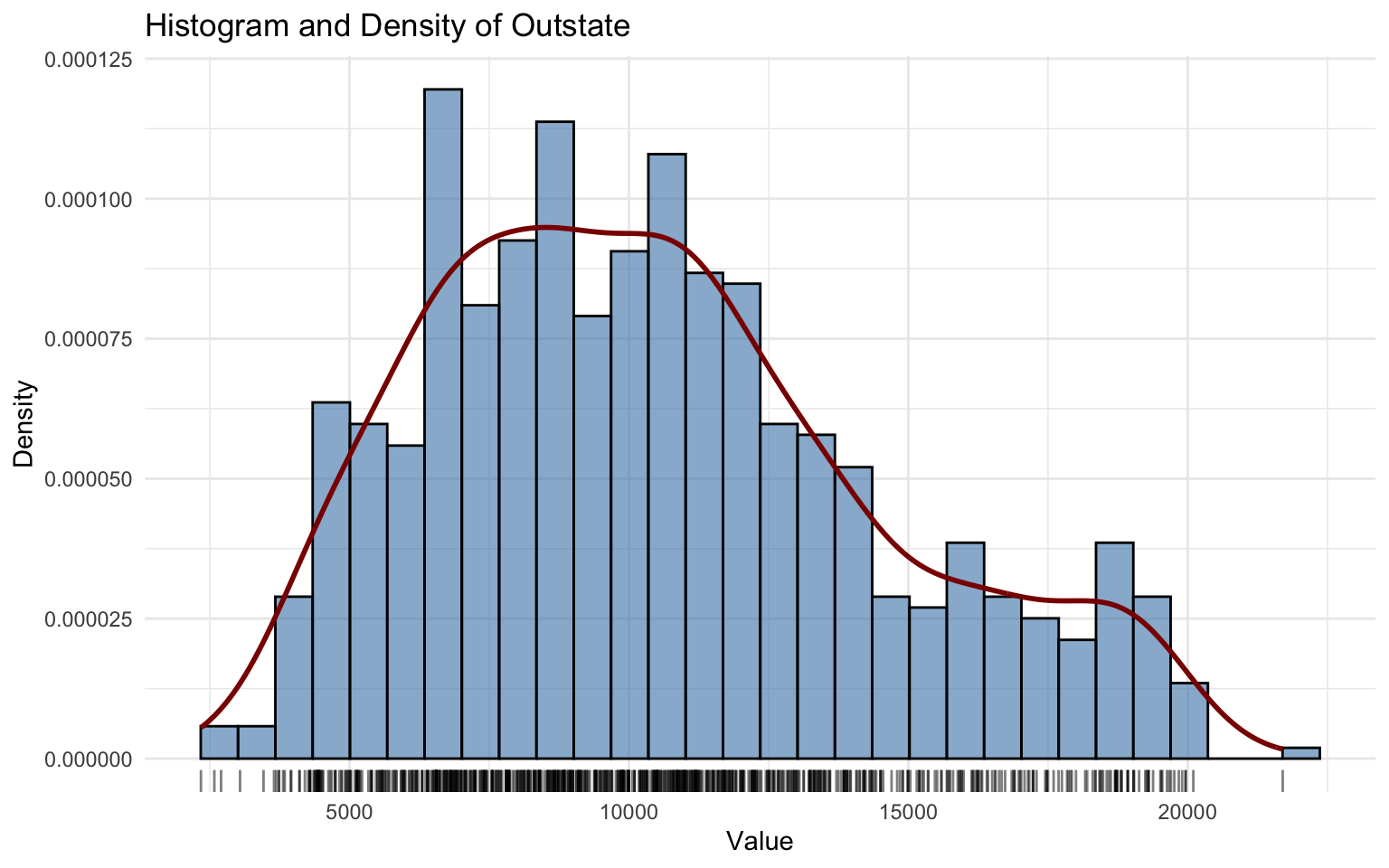
## EM iterations: 216 AIC: 15016.83 BIC: 15040.11 log-likelihood: -7503.42The Outstate variable is only mildly right-skewed.
The KDE reveals a structure that suggests a mixture distribution is appropriate. Therefore, a mixture of two Gamma distributions was selected, which successfully captures the observed pattern.
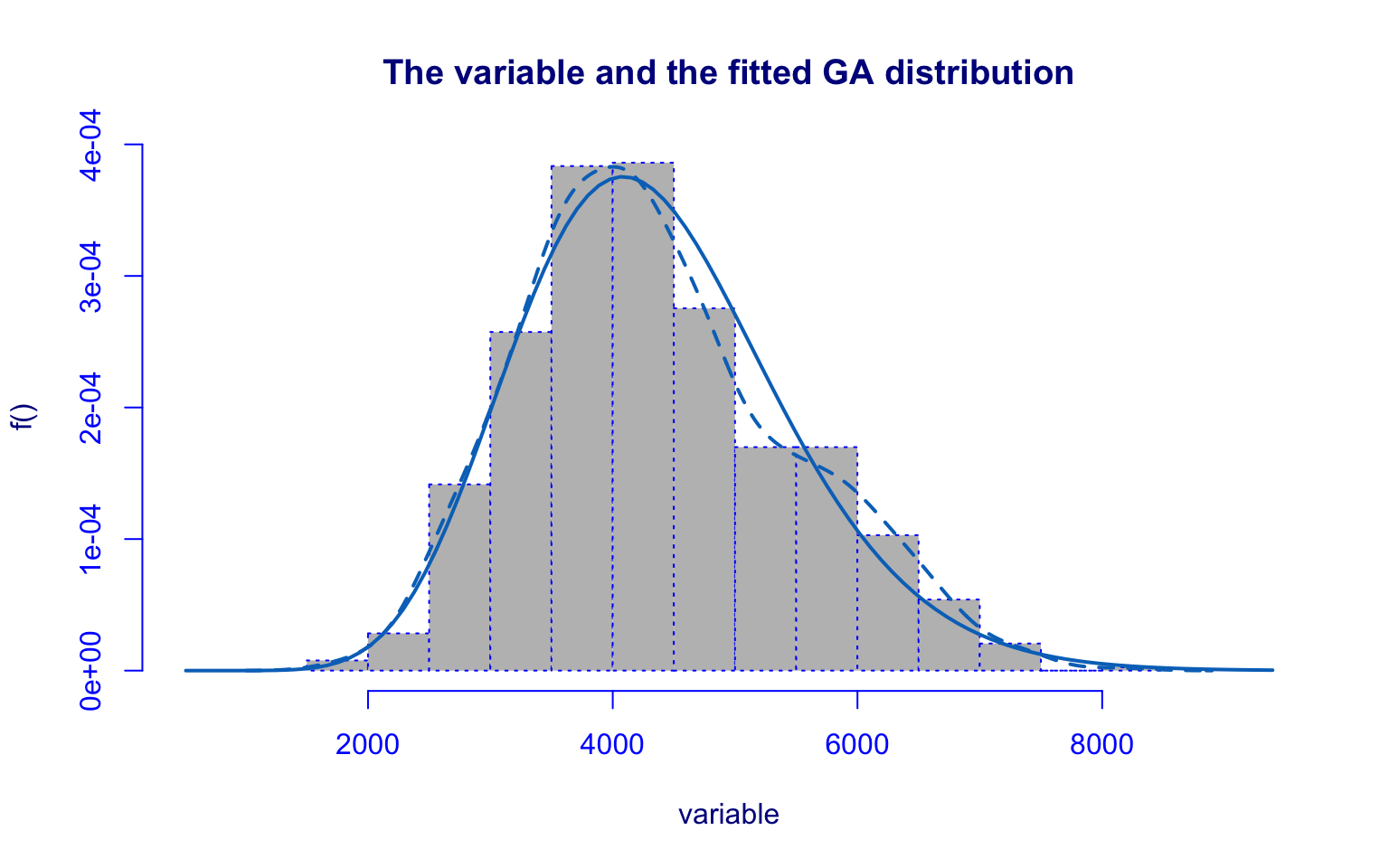
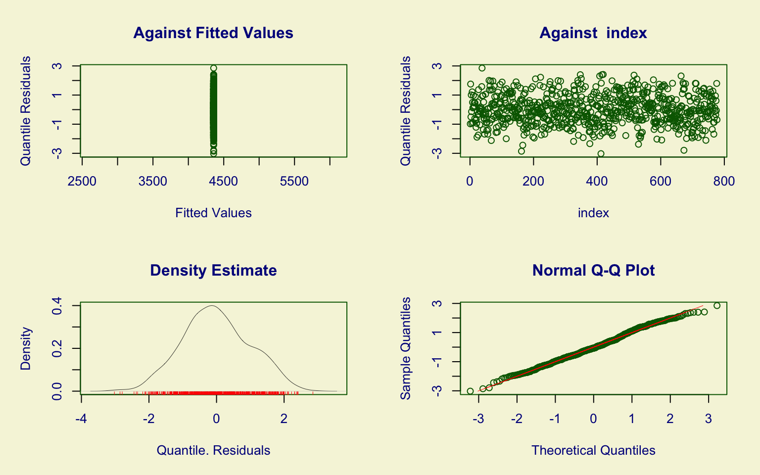
Room and board cost
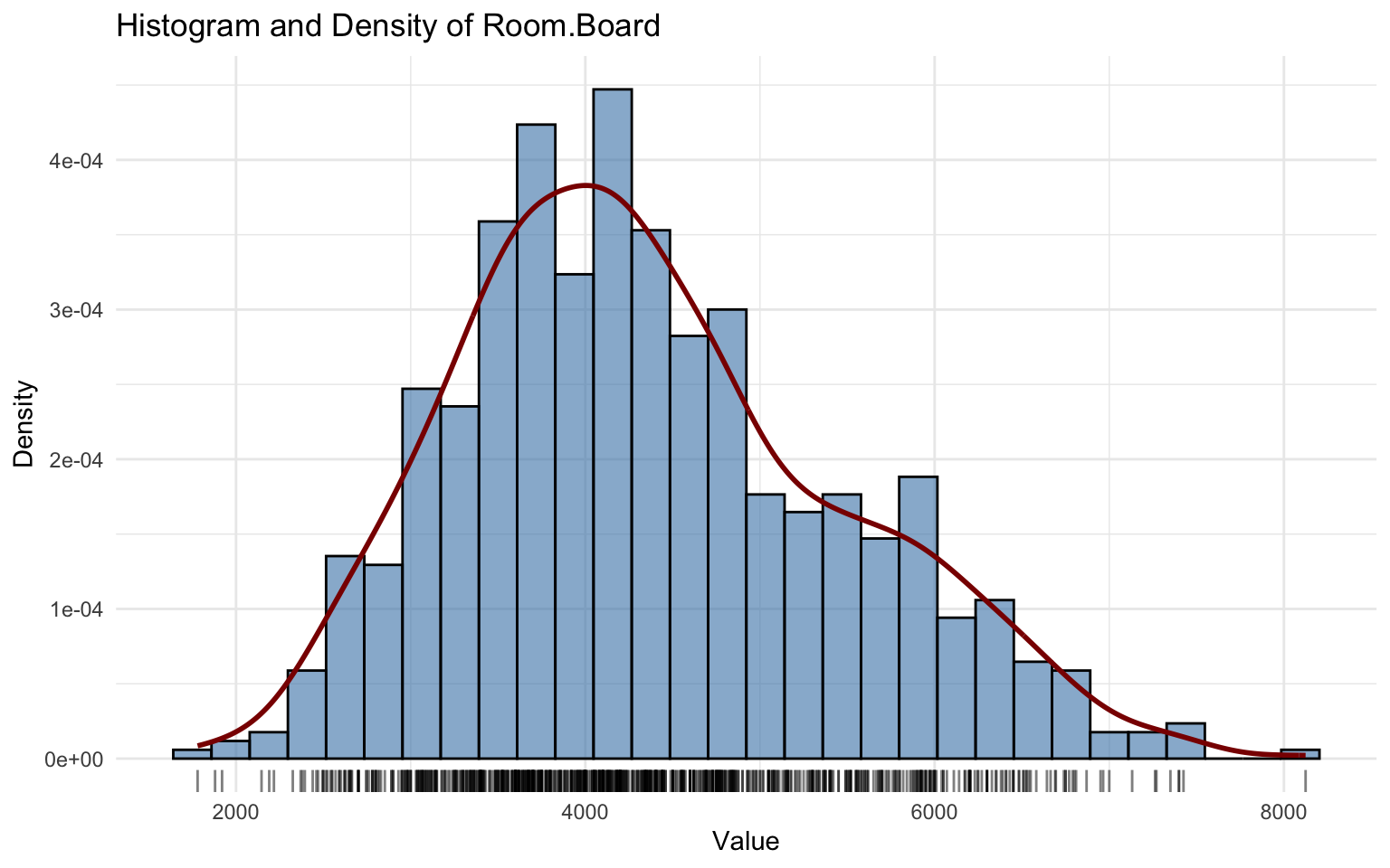
Distribution Fitting
## *******************************************************************
## Family:  c("GA", "Gamma")
##
## Call:  gamlssML(formula = y, family = DIST[i])
##
## Fitting method: "nlminb"
##
##
## Coefficient(s):
##              Estimate  Std. Error  t value   Pr(>|t|)
## eta.mu     8.37965953  0.00898582 932.5425 < 2.22e-16 ***
## eta.sigma -1.38438694  0.02510634 -55.1409 < 2.22e-16 ***
## ---
## Signif. codes:  0 '***' 0.001 '**' 0.01 '*' 0.05 '.' 0.1 ' ' 1
##
##  Degrees of Freedom for the fit: 2 Residual Deg. of Freedom   775
## Global Deviance:     13042.7
##             AIC:     13046.7
##             SBC:     13056
##
## Asymptotic one-sample Kolmogorov-Smirnov test
##
## data: unique(variable)
## D = 0.052409, p-value = 0.09587
## alternative hypothesis: two-sidedThe Room.Board variable shows a mild right skew.
The Gamma distribution provides a reasonably good fit:
- parameters \((\hat\mu, \hat\sigma)\) are significant;
- residual diagnostics are satisfactory, though minor imperfections appear in the upper tail and in the quantile residuals.
The Kolmogorov–Smirnov test (D = 0.052409, p-value = 0.09587) fails to reject the null hypothesis, supporting the adequacy of the Gamma model.
Cost of books
Distribution Fitting
## Gamma mixture model with 2 components
## comp1 comp2
## pi 0.8860079 0.1139921
## mu 536.3065083 651.0025872
## sd 100.0155646 368.3087167
## shape 28.7535156 3.1242187
## rate 0.0536140 0.0047991
##
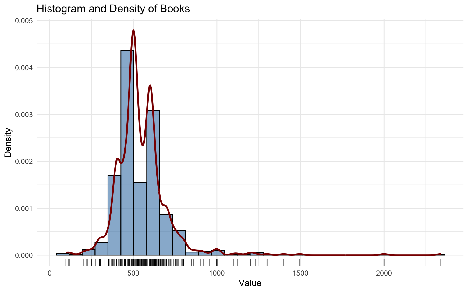
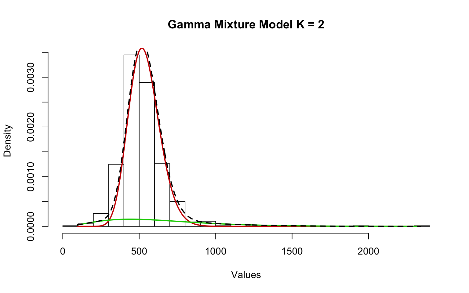
## EM iterations: 33 AIC: 9752.47 BIC: 9775.75 log-likelihood: -4871.24The behavior of the variable Books is unusual. The variable also shows a right-skewed distribution with several high- and low-value outliers. The KDE exhibits overfitting, which occurs when the smoothing parameter is too small.
The fitDist function in GAMLSS does not work well in this case, so a mixture of two Gamma distributions was applied.
Personal spending
Distribution Fitting
## *******************************************************************
## Family:  c("LOGNO", "Log Normal")
##
## Call:  gamlssML(formula = y, family = DIST[i])
##
## Fitting method: "nlminb"
##
##
## Coefficient(s):
##             Estimate  Std. Error  t value   Pr(>|t|)
## eta.mu     7.0850691   0.0174117 406.9153 < 2.22e-16 ***
## eta.sigma -0.7228953   0.0253673 -28.4971 < 2.22e-16 ***
## ---
## Signif. codes:  0 '***' 0.001 '**' 0.01 '*' 0.05 '.' 0.1 ' ' 1
##
##  Degrees of Freedom for the fit: 2 Residual Deg. of Freedom   775
## Global Deviance:     12091.8
##             AIC:     12095.8
##             SBC:     12105.2
##
## Asymptotic one-sample Kolmogorov-Smirnov test
##
## data: unique(variable)
## D = 0.21876, p-value = 1.202e-12
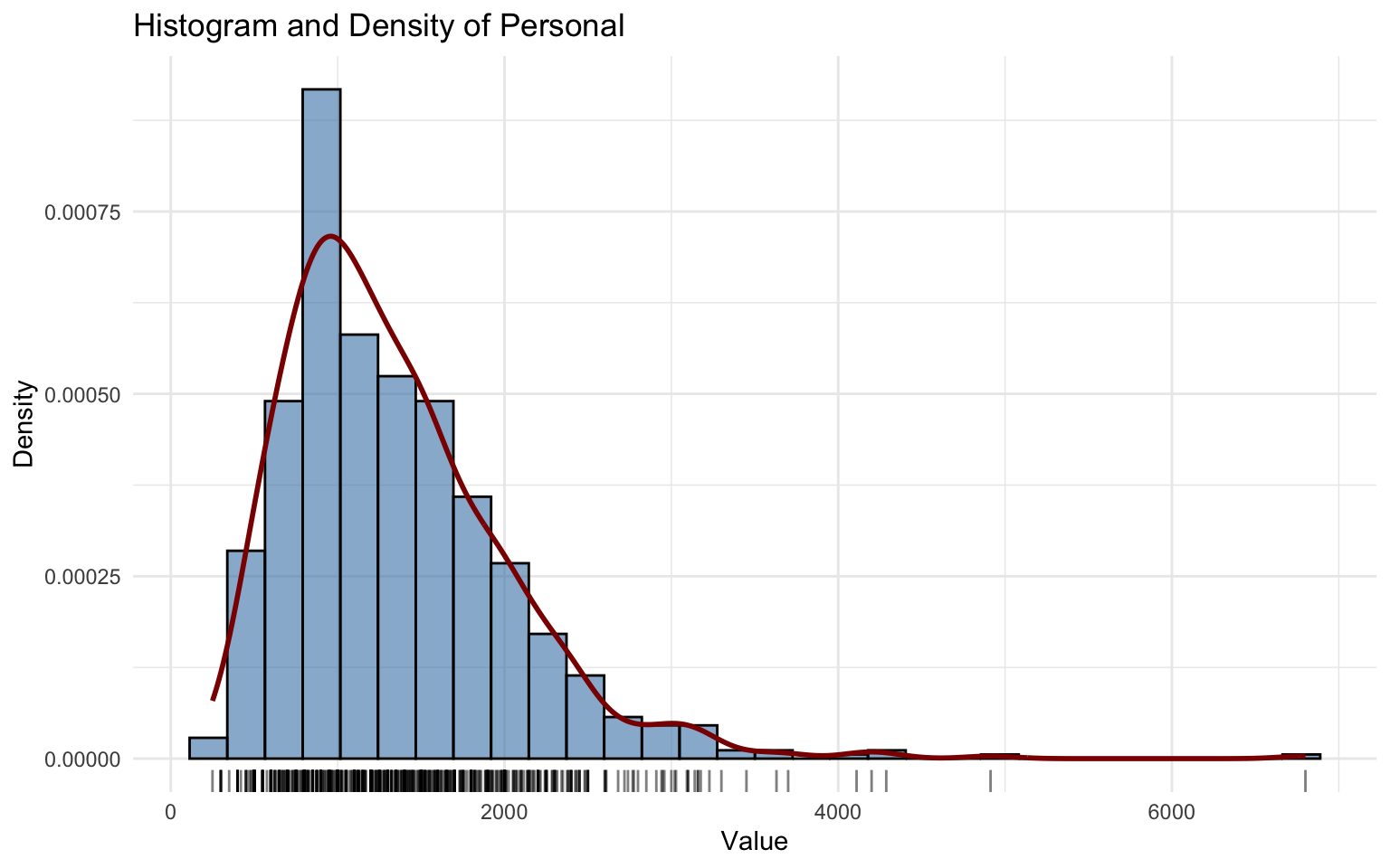
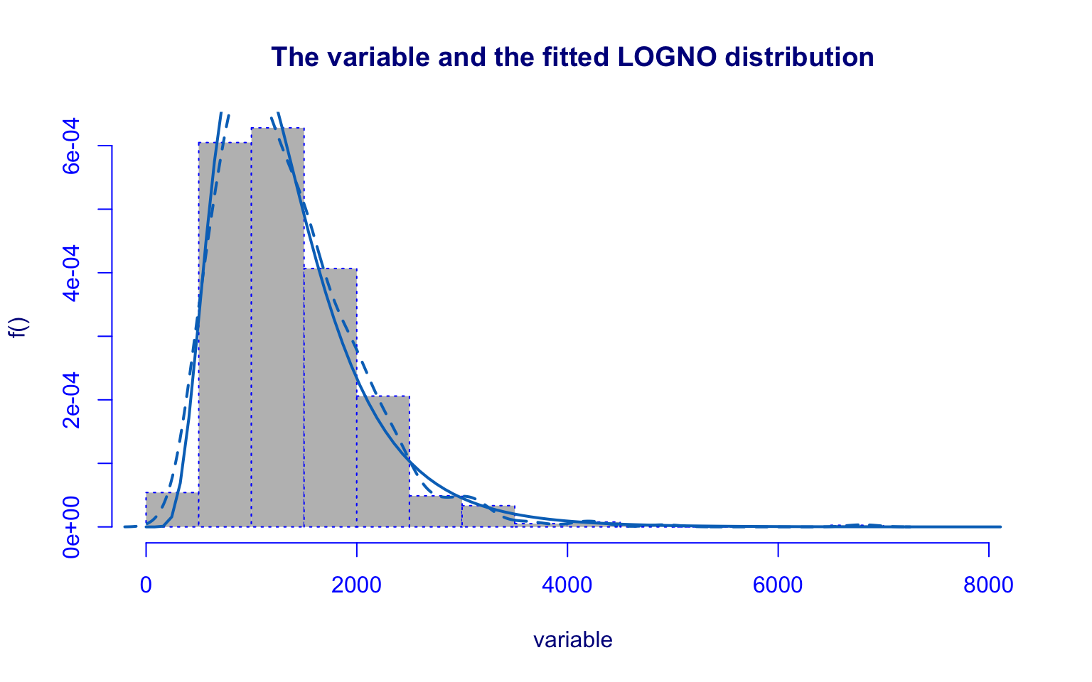
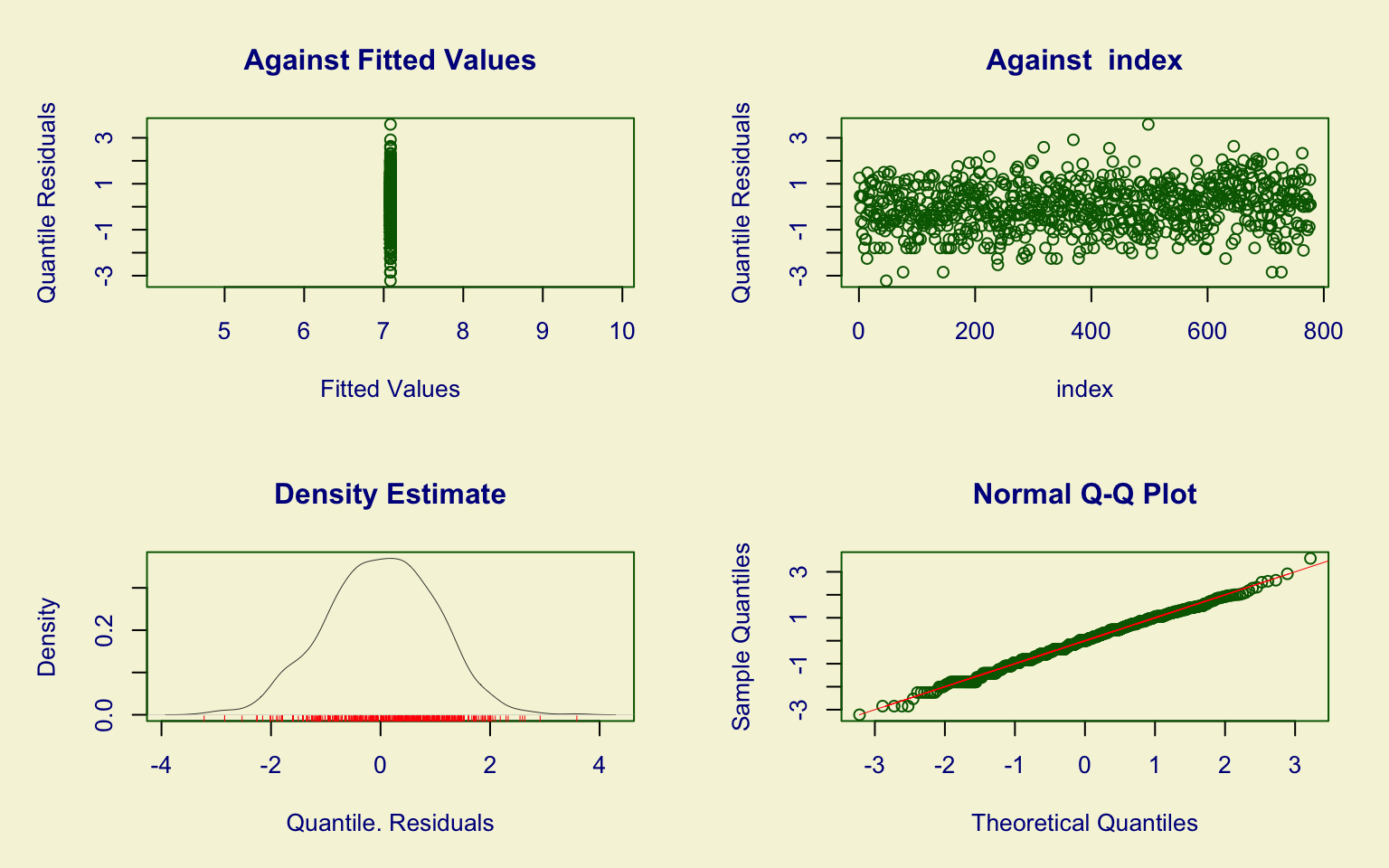
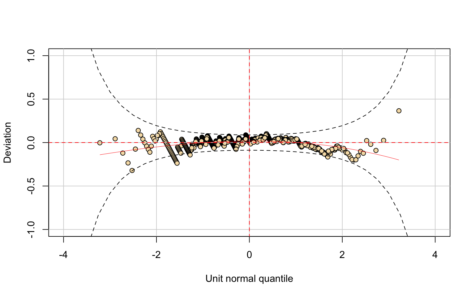
## alternative hypothesis: two-sidedThe Personal variable is right-skewed with outliers.
The Lognormal (LOGNO) distribution was tested but performed poorly:
- residual diagnostics deviate from normality;
- the Kolmogorov–Smirnov test confirms lack of fit.
Thus, the LOGNO model is not adequate for this variable.
Percentage of PhD
Distribution Fitting

## *******************************************************************
## Family:  c("GB1", "Generalized beta type 1")
##
## Call:  gamlssML(formula = y, family = DIST[i])
##
## Fitting method: "nlminb"
##
##
## Coefficient(s):
##             Estimate  Std. Error  t value   Pr(>|t|)
## eta.mu      1.913129    0.465327  4.11137 3.9332e-05 ***
## eta.sigma  -1.135873    0.220442 -5.15270 2.5677e-07 ***
## eta.nu     12.748402    4.141176  3.07845  0.0020808 **
## eta.tau   -13.549139    4.134993 -3.27670  0.0010503 **
## ---
## Signif. codes:  0 '***' 0.001 '**' 0.01 '*' 0.05 '.' 0.1 ' ' 1
##
##  Degrees of Freedom for the fit: 4 Residual Deg. of Freedom   769
## Global Deviance:     -746.751
##             AIC:     -738.751
##             SBC:     -720.15
##
## Exact one-sample Kolmogorov-Smirnov test
##
## data: unique(variable)
## D = 0.27364, p-value = 1.609e-05
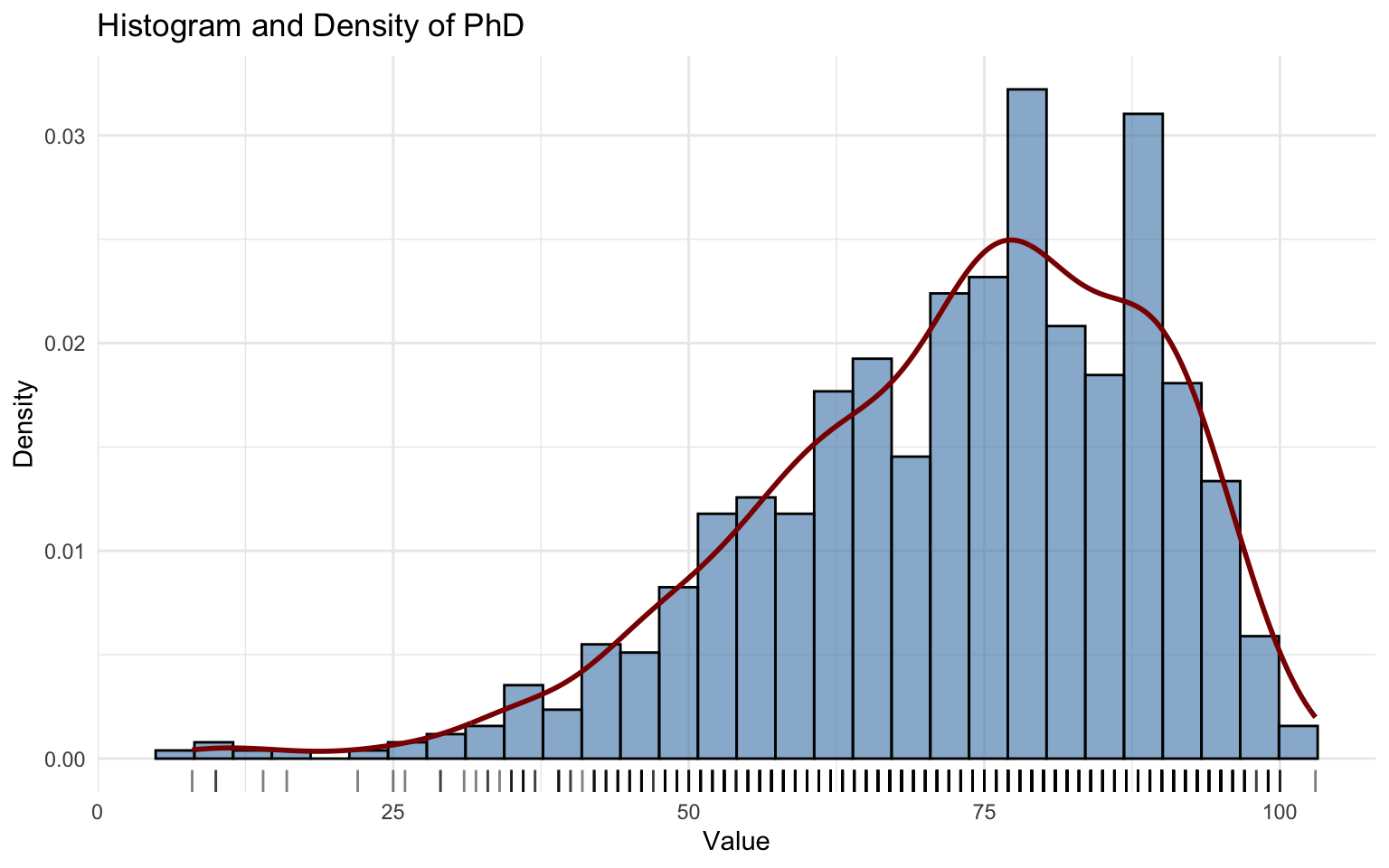
## alternative hypothesis: two-sidedThe PhD variable was fitted using the Generalized Beta type 1 (GB1). However, the model does not fit well, as shown by residual diagnostics and the Kolmogorov–Smirnov test.
Moreover, the fitting procedure raised convergence warnings, indicating potential instability in parameter estimation.
Percentage of terminal degrees
Distribution Fitting
## *******************************************************************
## Family:  c("BE", "Beta")
##
## Call:  gamlssML(formula = y, family = BE)
##
## Fitting method: "nlminb"
##
##
## Coefficient(s):
##             Estimate  Std. Error  t value   Pr(>|t|)
## eta.mu     1.3457668   0.0318862  42.2053 < 2.22e-16 ***
## eta.sigma -0.5809269   0.0339839 -17.0942 < 2.22e-16 ***
## ---
## Signif. codes:  0 '***' 0.001 '**' 0.01 '*' 0.05 '.' 0.1 ' ' 1
##
##  Degrees of Freedom for the fit: 2 Residual Deg. of Freedom   761
## Global Deviance:     -1010.92
##             AIC:     -1006.92
##             SBC:     -997.65
##
## Exact one-sample Kolmogorov-Smirnov test
##
## data: unique(variable)
## D = 0.30976, p-value = 5.949e-06
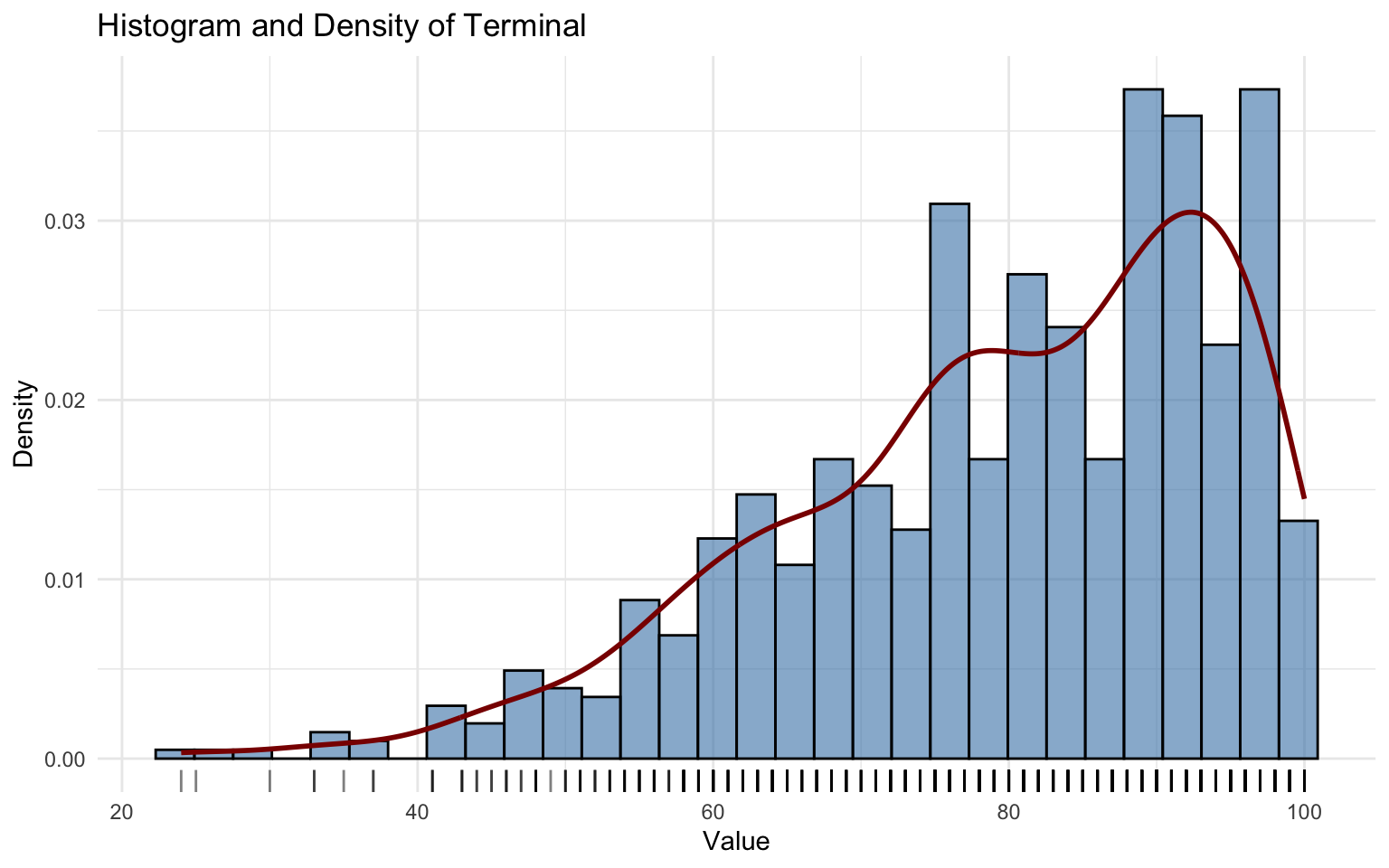
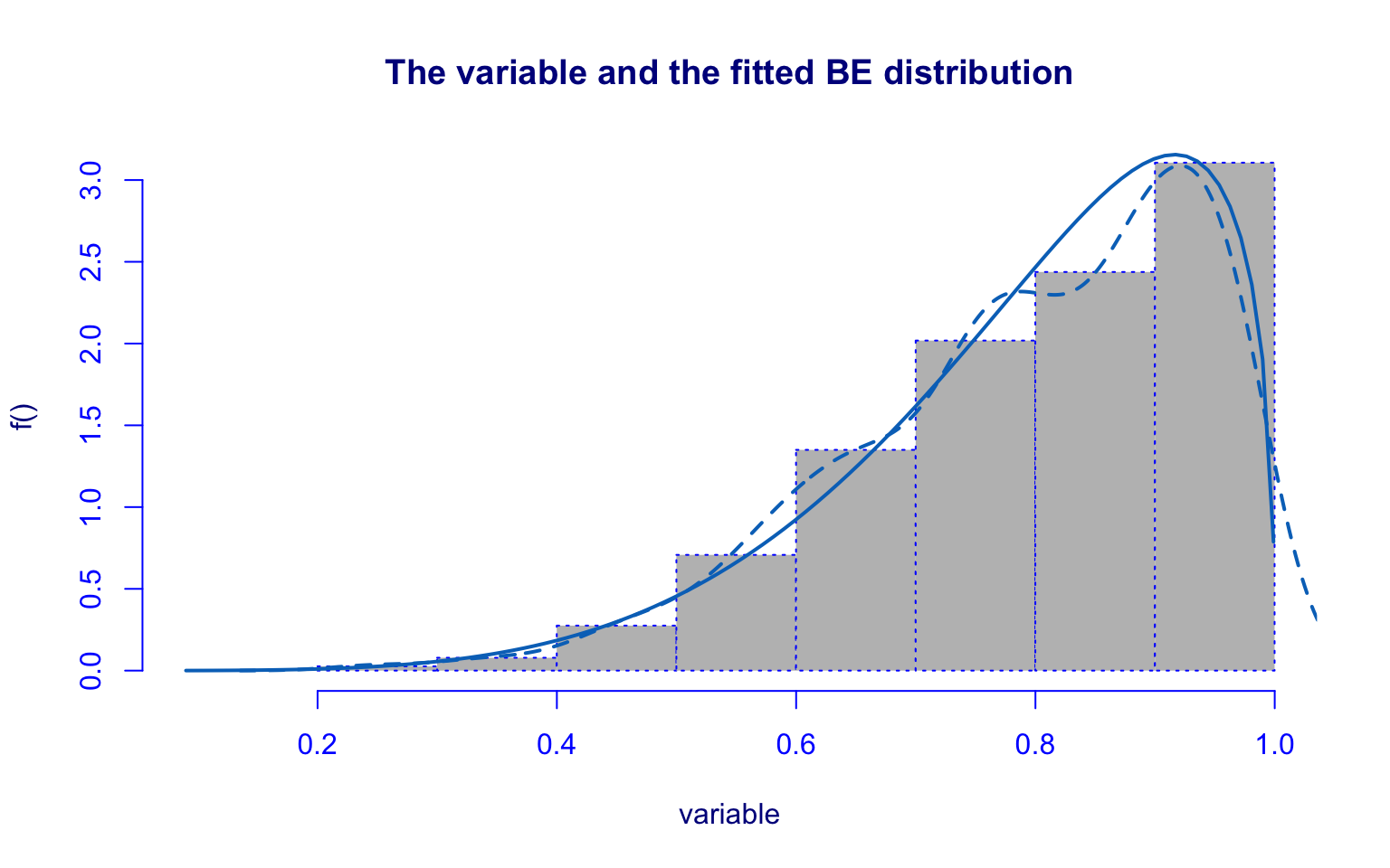
## alternative hypothesis: two-sidedThe Terminal variable was modeled with the Beta (BE) distribution.
Although the parameter estimates are reasonable, residual diagnostics show values outside the 95% confidence interval and the Kolmogorov–Smirnov test rejects the null hypothesis.
Hence, the BE model is not a suitable fit.
Student-faculty ratio
Distribution Fitting
## *******************************************************************
## Family:  c("GB1", "Generalized beta type 1")
##
## Call:  gamlssML(formula = y, family = DIST[i])
##
## Fitting method: "nlminb"
##
##
## Coefficient(s):
##             Estimate  Std. Error  t value   Pr(>|t|)
## eta.mu     -0.542462    0.177567 -3.05496  0.0022509 **
## eta.sigma   0.275956    0.246668  1.11873  0.2632547
## eta.nu    -11.963796    2.635678 -4.53917 5.6475e-06 ***
## eta.tau     1.860055    0.200696  9.26803 < 2.22e-16 ***
## ---
## Signif. codes:  0 '***' 0.001 '**' 0.01 '*' 0.05 '.' 0.1 ' ' 1
##
##  Degrees of Freedom for the fit: 4 Residual Deg. of Freedom   773
## Global Deviance:     -2857.75
##             AIC:     -2849.75
##             SBC:     -2831.13
##
## Asymptotic one-sample Kolmogorov-Smirnov test
##
## data: unique(variable)
## D = 0.17268, p-value = 6.609e-05
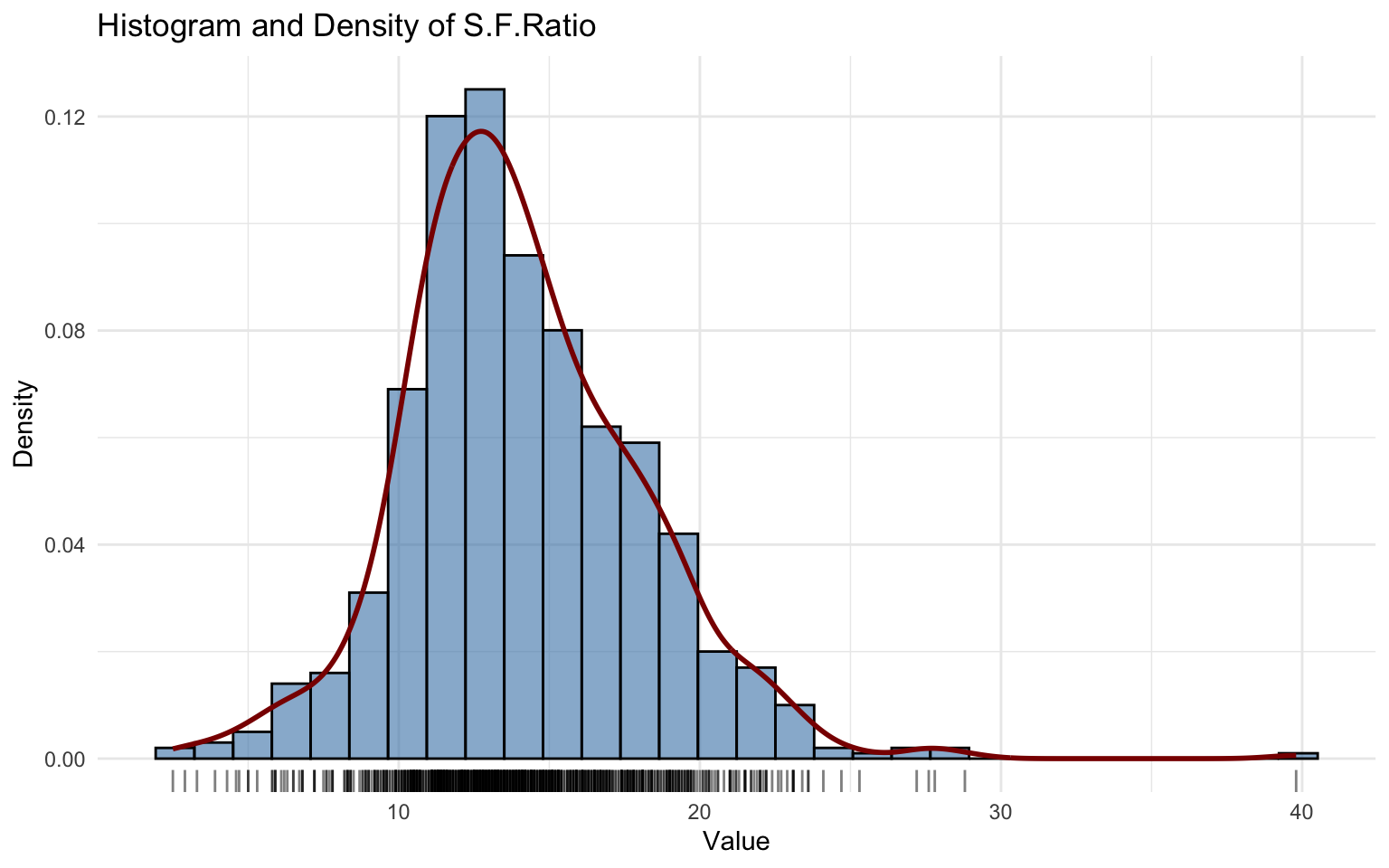
## alternative hypothesis: two-sidedThe S.F.Ratio variable was modeled using Generalized beta type 1 (GB1), but both residual analysis and the Kolmogorov–Smirnov test show poor fit.
This indicates that the GB1 distribution does not adequately describe the data.
Percentage of student donors
Distribution Fitting
## *******************************************************************
## Family:  c("BEo", "Beta original")
##
## Call:  gamlssML(formula = y, family = DIST[i])
##
## Fitting method: "nlminb"
##
##
## Coefficient(s):
##            Estimate  Std. Error  t value   Pr(>|t|)
## eta.mu    0.8757280   0.0478023  18.3198 < 2.22e-16 ***
## eta.sigma 2.0962922   0.0514518  40.7428 < 2.22e-16 ***
## ---
## Signif. codes:  0 '***' 0.001 '**' 0.01 '*' 0.05 '.' 0.1 ' ' 1
##
##  Degrees of Freedom for the fit: 2 Residual Deg. of Freedom   773
## Global Deviance:     -1151.36
##             AIC:     -1147.36
##             SBC:     -1138.05
##
## Exact one-sample Kolmogorov-Smirnov test
##
## data: unique(variable)
## D = 0.26808, p-value = 0.0002684
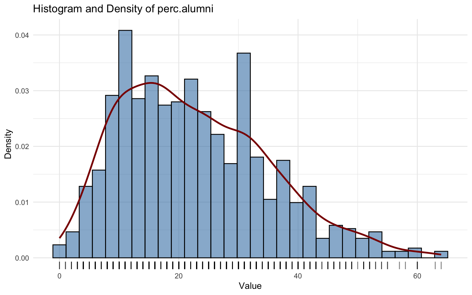
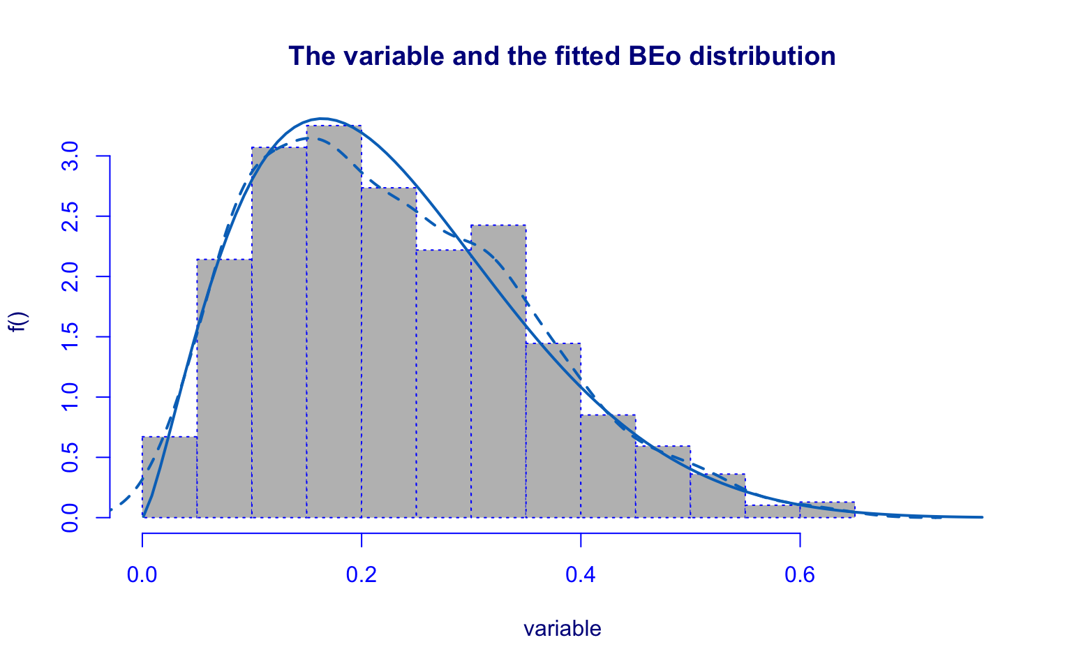
## alternative hypothesis: two-sidedThe perc.alumni variable was modeled with the Beta-original (BEo) distribution.
Although the KDE and fitted distribution show some alignment, diagnostic checks reveal important issues:
- quantile residuals exhibit kurtosis;
- the Kolmogorov–Smirnov test (D = 0.26808, p-value = 0.0002684) rejects the null hypothesis.
Thus, the BEo distribution provides only a partial description of the data.
Instructional expenditure
Distribution Fitting
## *******************************************************************
## Family:  c("BCPE", "Box-Cox Power Exponential")
##
## Call:  gamlssML(formula = y, family = DIST[i])
##
## Fitting method: "nlminb"
##
##
## Coefficient(s):
##               Estimate   Std. Error   t value   Pr(>|t|)
## eta.mu    8410.5398898  116.6109377  72.12479 < 2.22e-16 ***
## eta.sigma   -0.9622819    0.0307236 -31.32062 < 2.22e-16 ***
## eta.nu      -0.5226112    0.0815880  -6.40549 1.4989e-10 ***
## eta.tau      0.4273583    0.0771043   5.54260 2.9802e-08 ***
## ---
## Signif. codes:  0 '***' 0.001 '**' 0.01 '*' 0.05 '.' 0.1 ' ' 1
##
##  Degrees of Freedom for the fit: 4 Residual Deg. of Freedom   773
## Global Deviance:     14843
##             AIC:     14851
##             SBC:     14869.6
##
## Asymptotic one-sample Kolmogorov-Smirnov test
##
## data: unique(variable)
## D = 0.026043, p-value = 0.6939
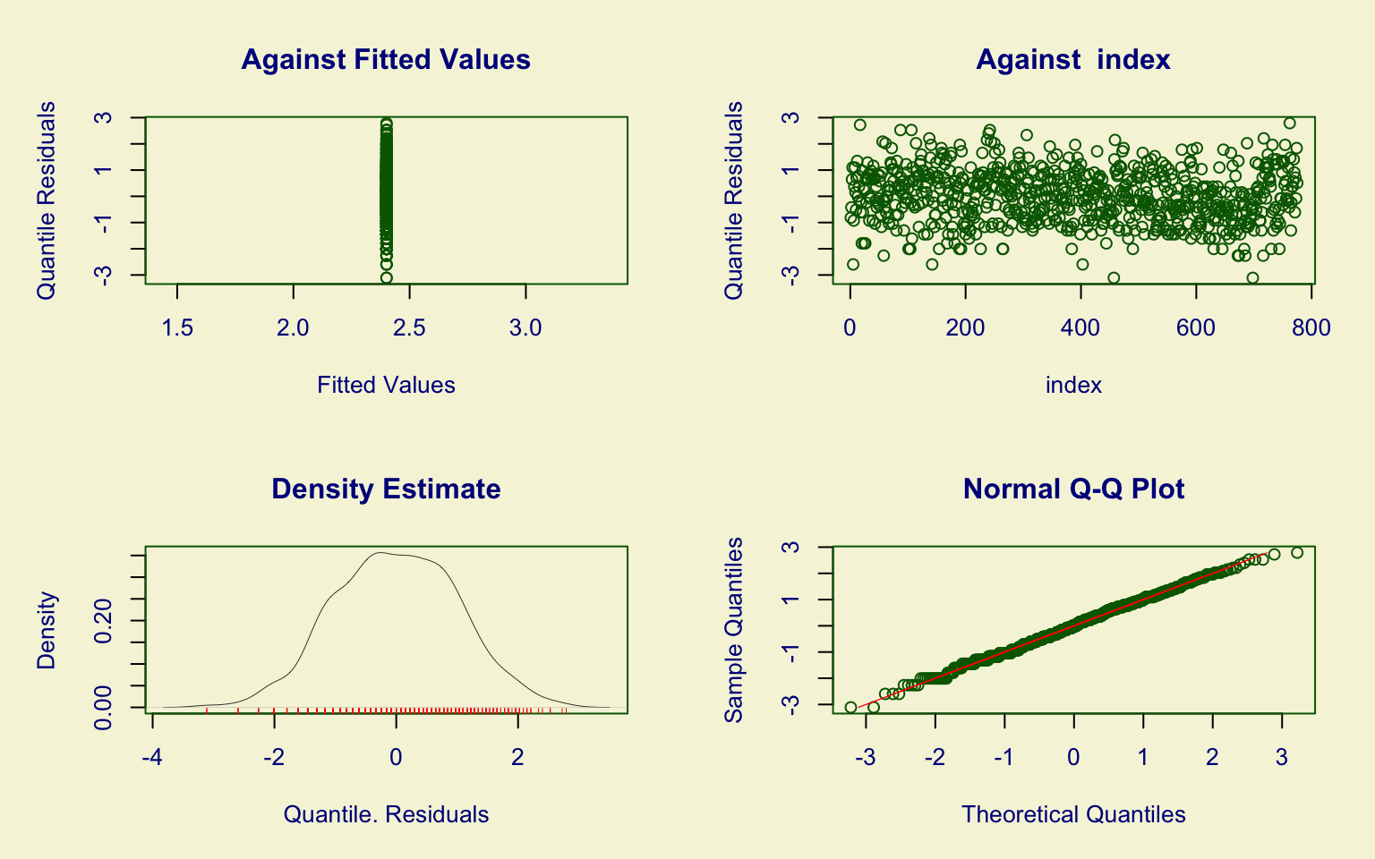
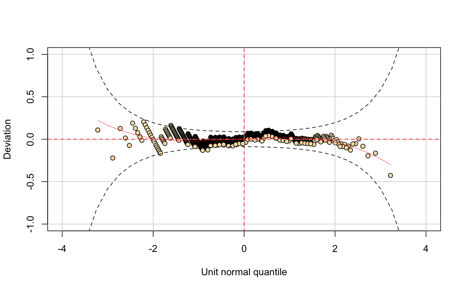
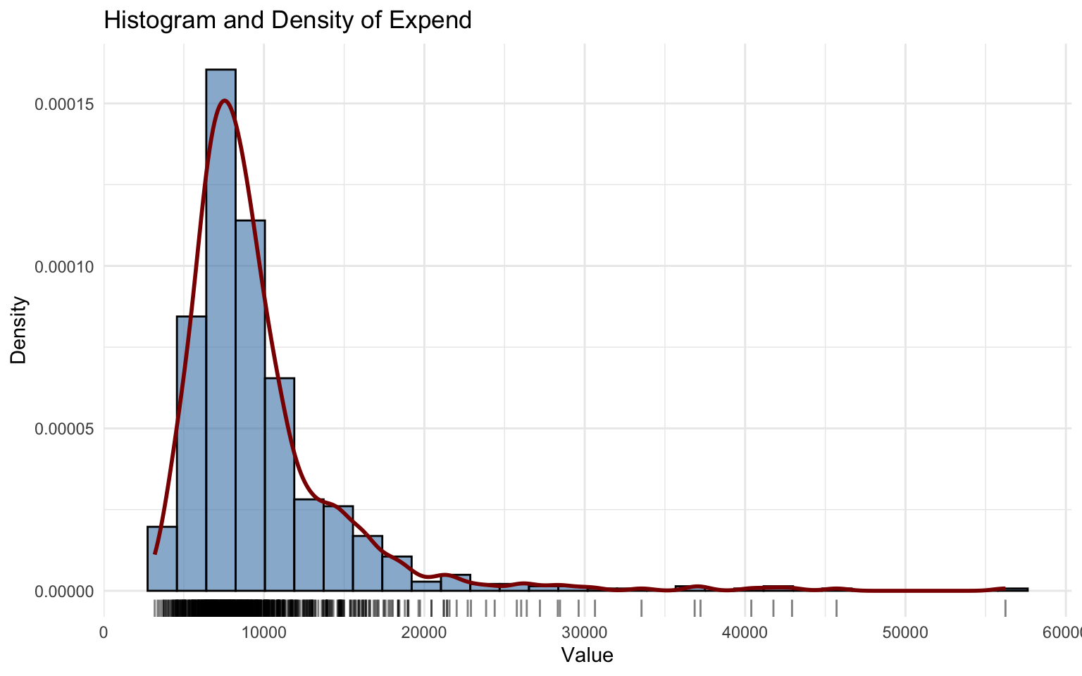
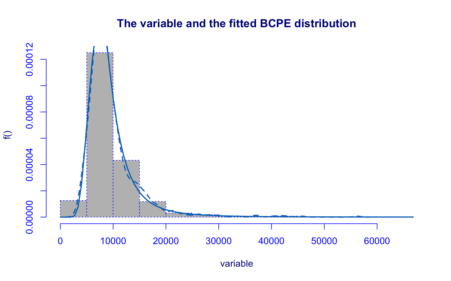
## alternative hypothesis: two-sidedThe Expend variable is well modeled by the Box-Cox Power Exponential (BCPE).
All parameters are highly significant, residuals follow approximately a \(N(0,1)\) distribution, and the Kolmogorov–Smirnov test (D = 0.026043, p-value = 0.6939) fails to reject the null hypothesis.
This indicates a very good fit.
Graduation rate
Distribution Fitting
## *******************************************************************
## Family:  c("GB1", "Generalized beta type 1")
##
## Call:  gamlssML(formula = y, family = DIST[i])
##
## Fitting method: "nlminb"
##
##
## Coefficient(s):
##            Estimate  Std. Error  t value   Pr(>|t|)
## eta.mu    -0.380954    0.194370 -1.95994  0.0500029 .
## eta.sigma  0.400045    0.141763  2.82193  0.0047736 **
## eta.nu    -1.986350    0.384539 -5.16554 2.3974e-07 ***
## eta.tau    1.810241    0.201202  8.99712 < 2.22e-16 ***
## ---
## Signif. codes:  0 '***' 0.001 '**' 0.01 '*' 0.05 '.' 0.1 ' ' 1
##
##  Degrees of Freedom for the fit: 4 Residual Deg. of Freedom   762
## Global Deviance:     -602.839
##             AIC:     -594.839
##             SBC:     -576.274
##
## Exact one-sample Kolmogorov-Smirnov test
##
## data: unique(variable)
## D = 0.19321, p-value = 0.004664
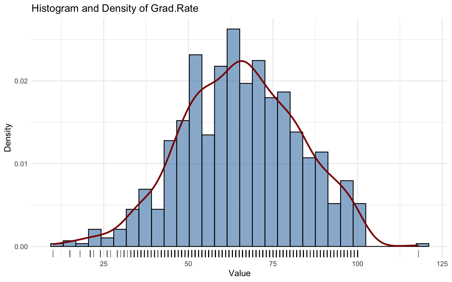
## alternative hypothesis: two-sidedThe Grad.Rate variable is slightly left-skewed.
The Generalized beta type 1 (GB1) distribution provides a reasonable graphical fit, with residuals showing no major problems.
However, the Kolmogorov–Smirnov test (D = 0.19321, p-value = 0.004664) rejects the null hypothesis, suggesting that the GB1 model does not fully capture the distribution.